What Is Table Array in Excel VLOOKUP?

What Is Table Array Argument in VLOOKUP Function?

The Table Array argument in the Excel VLOOKUP function is used to find and look up the desired values in the form of an array in the table. While using the VLOOKUP function, we need to set a data range where we’ll look up our value. This range is called the Table Array.

Syntax:

VLOOKUP(lookup_value, table_array, col_index_num, [range_lookup])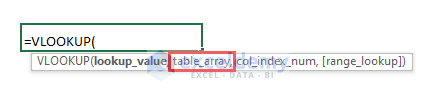Arguments:

lookup_value: The value used to look up.

table_array: The selected range in which you want to find the lookup value and the return value. It is also called the Table Array.

col_index_num: The number of column within your selected range that contains the return value.

[range_lookup]: FALSE or 0 for an exact match, TRUE or 1 for an approximate match.

Using the Table Array Argument in Excel VLOOKUP: 3 Useful Examples

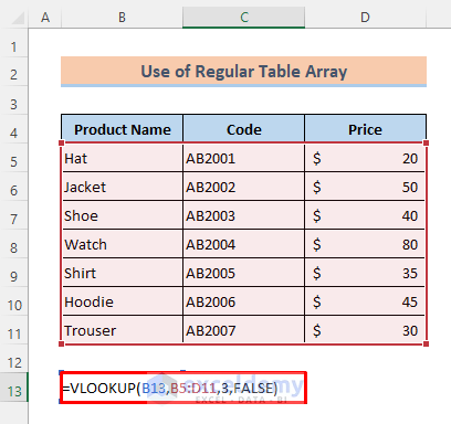
Example 1 – Regular Table Array in the Same Excel Worksheet

Steps:

⏩ Enter the following formula in Cell C13:

B5:B13 is the Table Array.

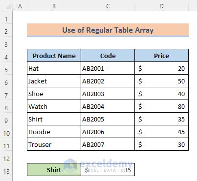
⏩ Press Enter to get the output.

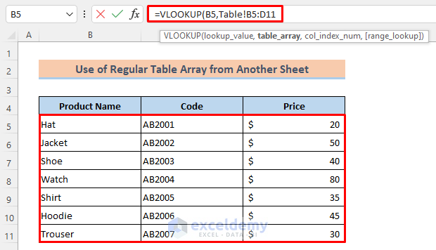
Example 2 – Regular Table Array from Another Excel Worksheet

Steps:

⏩ Enter the following formula-

⏩ Click on the worksheet name where the data range is located.

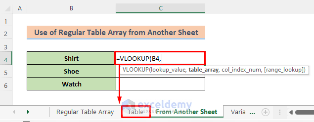
⏩ Select the data range B5:D11 from this sheet.

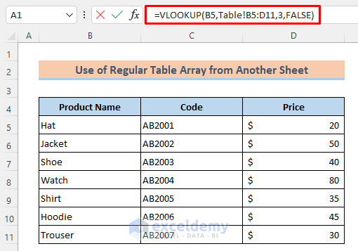
⏩ Complete the other arguments input as shown in the previous example.

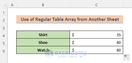
⏩ Press Enter and drag the Fill Handle icon.

Read More: How to Find Table Array in Excel

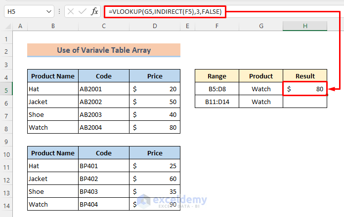
Example 3 – Variable Table Array

Steps:

⏩ Activate Cell H5.

⏩ Enter the following formula.

⏩ Press Enter.

⏩ Drag the Fill Handle icon to copy the formula to the remaining cells.

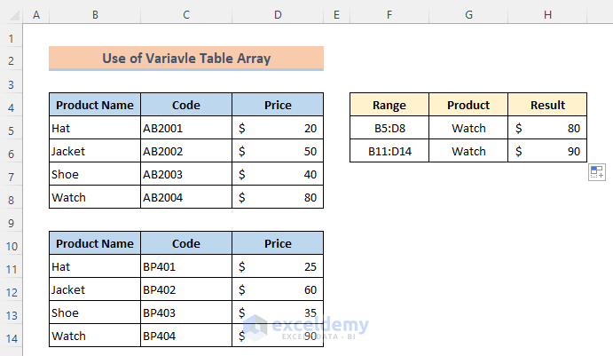
⏬ Formula Breakdown:

➤ INDIRECT(F5)
The INDIRECT function will return the reference to a range like-
{“Hat”,”AB2001″,20;”Jacket”,”AB2002″,50;”Shoe”,”AB2003″,40;”Watch”,”AB2004″,80}

➤ VLOOKUP(G5,INDIRECT(F5),3,FALSE)
The VLOOKUP function will give the corresponding result from the range. For Cell G5 it returns as-
80

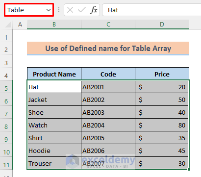
Example 4 – Use Defined Names for Table Array

Steps:

⏩ Select the data range B5:D11.

⏩ Press the cell name box and enter a name. We have set the name ‘Table’.

⏩ Press Enter.

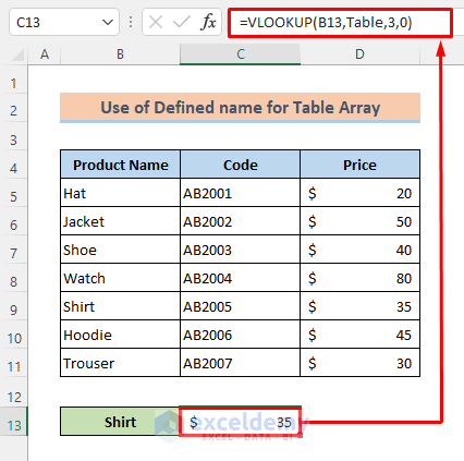
⏩ Activate Cell C13.

⏩ Enter the following formula-

⏩ Press Enter.

Read More: How to Name a Table Array in Excel

Why Is Excel VLOOKUP Not Working and How to Resolve

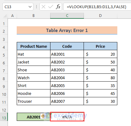
Reason 1 – The Lookup Value is Not in the First Column in the Table Array

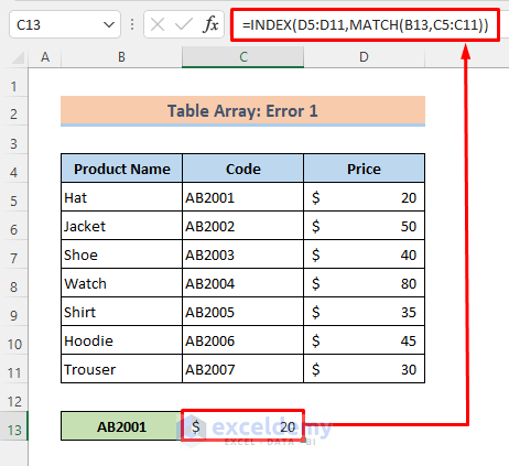
One limitation of VLOOKUP is that it can only look for values from the left-most column in the table array. So If your lookup value is not in the first column of the array you will see the #N/A error. In the image below, our lookup value is from the second column of the table array that’s why it is showing #N/A.

Solution:

The solution to this problem is not to use VLOOKUP. Using a combination of the INDEX and MATCH functions is an alternative to VLOOKUP.

Steps:

⏩ In Cell C13, enter the formula-

⏩ Press Enter button to get the result.

⏬ Formula Breakdown:

➤ MATCH(B13,C5:C11)
The MATCH function will locate the position of the lookup value from the array C5:C11 that will return as-
1

➤ INDEX(D5:D11,MATCH(B13,C5:C11))
The INDEX function will return the value according to the location given by the MATCH function that is-
20

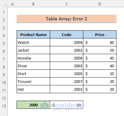
Reason 2 – The Lookup Value is Smaller Than the Smallest Value in the Table Array

If the lookup value becomes smaller than the lowest value of the array then the VLOOKUP function will return an error too. In the image below, all of our arguments are right but the lookup value is smaller, so it is shows an error.

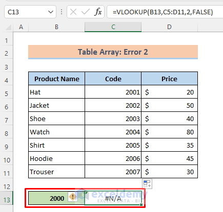
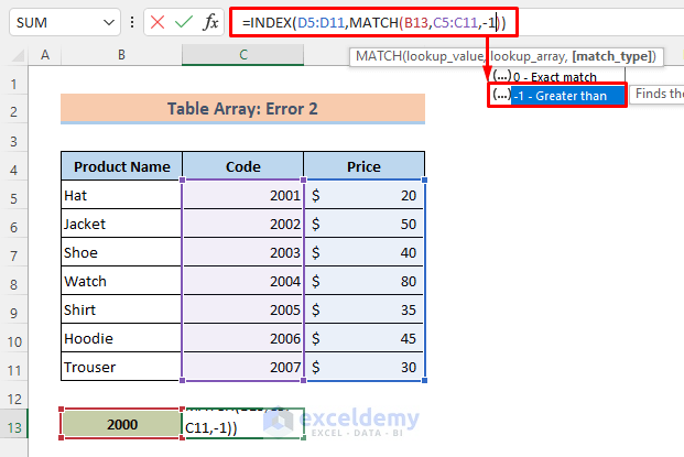
Solution:

The first solution is to Correct the lookup value as necessary. And the second solution is to use set the match type (-1) Greater Than in the MATCH function like the image below. But for that, the array should be in descending order.

Steps:

⏩ Select the data range D5:D11.

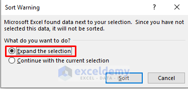
⏩ Click as follows: Home > Editing > Sort & Filter > Sort Largest to Smallest.

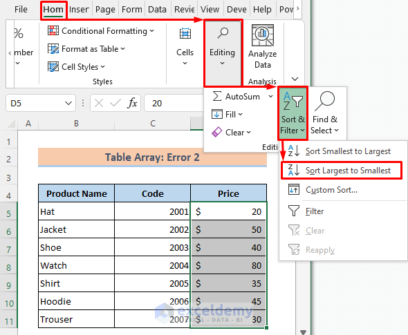
⏩ Mark Expand the selection.

⏩ Press Sort.

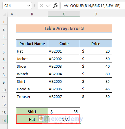
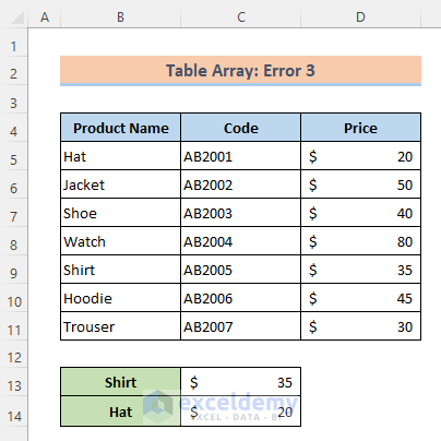
Reason 3 – Table Reference Not Locked

When searching for multiple lookup values to return different information about a record, if you don’t lock the table reference then you may get an error while using the Fill Handle tool to copy the formula as shown in the image below.

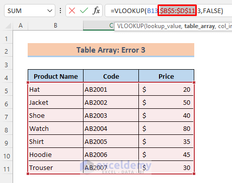
Solution:

Lock the table array reference to solve this issue.

Steps:

⏩ Press on the reference within the formula.

⏩ Press the F4 key to change the reference from relative to an absolute reference.

Read More: How to Lock Table Array in Excel

Download Practice Book

Related Articles

• How to Use VLOOKUP Table Array Based on Cell Value in Excel
• How to Expand Table Array in Excel

<< Go Back to Table Array in Excel | Excel VLOOKUP Function | Excel Functions | Learn Excel