Method 1 – Using Name Manager to Find Table Array in Excel
Steps:
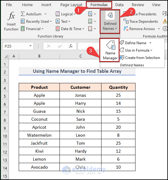
- Go to the Formulas tab.
- Click on the Defined Names group drop-down.
- Select Name Manager from the available options.
- The Name Manager dialog box opens up.
- We can see our named range in the list. Select MyTable.
- Click on the upside arrow beside the box of Refers To:
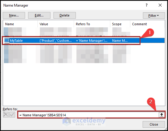
- It opens the Name Manager – Refers To: input box.
- We can see the cell range of MyTable in the box. Cells in the B4:D14 get bounded by a green dashed line to indicate the named range in the worksheet.
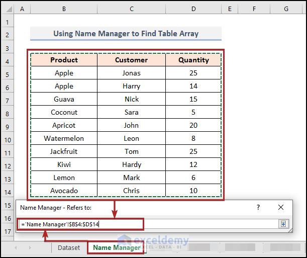
Note: Name Manager in the input box refers to the name of the current worksheet. See the picture above for a better understanding.
Method 02 – Utilizing Go To Feature to Find Table Array in Excel
Steps:
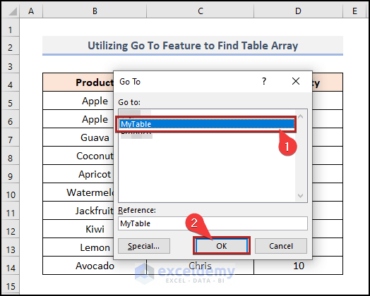
- Press CTRL + G on your keyboard.
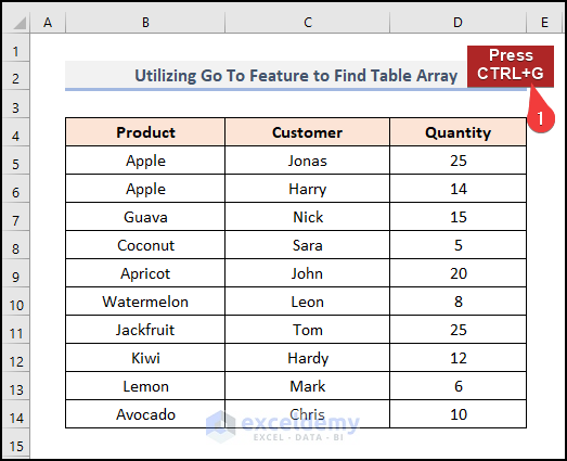
- It opens the Go To dialog box.
- Select MyTable under the section of Go To:.
- Click OK.
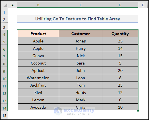
- It highlights the cell range of the named range MyTable, which is B4:D14. Creates a green solid line around the range.
- Find our table array in Excel.
Method 03 – Find Table Array in VLOOKUP in Excel
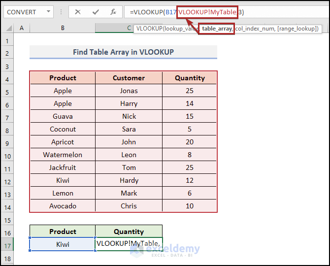
- In cell C17, we determined the number of sales of Kiwis using VLOOKUP.
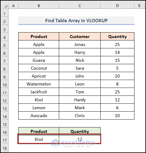
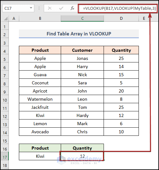
- Select cell C17 and we can see the formula below.
=VLOOKUP(B17,VLOOKUP!MyTable,3)
B17 refers to Kiwi. Then, VLOOKUP!MyTable indicates the table_array argument. And 3 means the col_index-num.
See the table_array as a name, but if we want to know the cell range of the named range, what should we do?
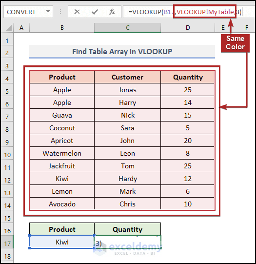
- Put the cursor on VLOOKUP!MyTable in the Formula Bar, it highlights the table_array argument. So, we can be sure this is the table array in our formula.
- It resembles the same color in VLOOKUP!MyTable and cells in the B4:D14 range. Both feature red color, so we can be sure that they are the same entity.
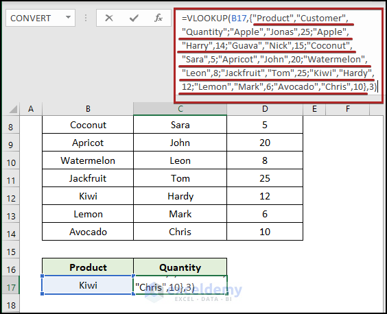
- Select the table_array in the Formula Bar and press F9 on your keyboard. You can see the argument in array form.
Method 4 – Find Table Array in HLOOKUP in Excel
Steps:
- Select cell C17.
- Find the formula in the Formula Bar like below.
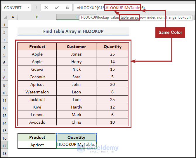
=HLOOKUP(C16,HLOOKUP!MyTable,6)
C16 resembles Product which is the lookup_value. Besides, HLOOKUP!MyTable serves as table_array argument. 6 represents the row_index_num.
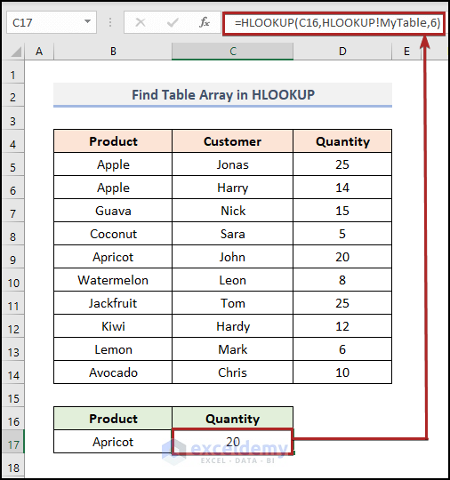
- When we put the cursor on HLOOKUP!MyTable in the Formula Bar, it highlights the table_array argument. So, we can be sure this is the table array in our formula.
- It resembles the same color in HLOOKUP!MyTable and cells in the B4:D14 range. Feature red color. From that, we can be sure that they are the same entity.
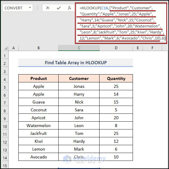
- Select the table_array in the Formula Bar and press F9 on your keyboard. You can see the argument in array form.
How to Find Lookup Array in XLOOKUP in Excel
Steps:
- Select cell C17.
- Find the formula in the Formula Bar like below.
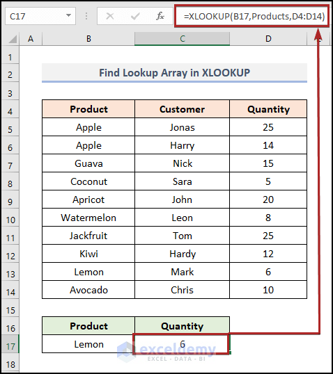
=XLOOKUP(B17,Products,D4:D14)
B17 represents Lemon which is the lookup_value. Products and D4:D14 serve as the lookup_array and return_array.
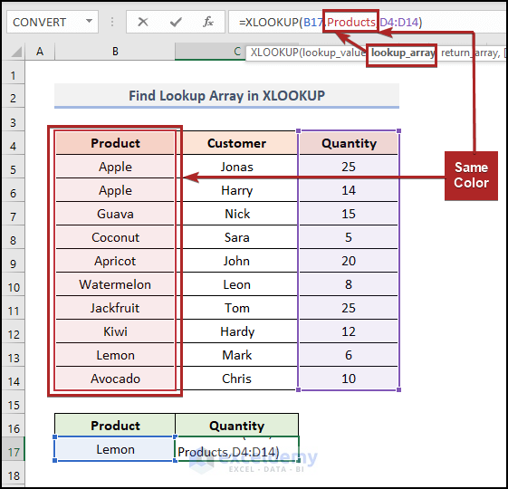
- When we put the cursor on Products in the Formula Bar, it highlights the lookup_array argument.
- It resembles the same color in Products and cells in the B4:B14 range. Feature red color, so we can be sure that they are the same entity.
- Select the Products in the Formula Bar and press F9 on your keyboard. You can see the argument in array form.
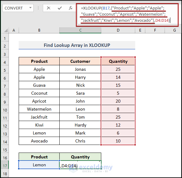
That’s how we can find the lookup array in XLOOKUP in Excel.
Download Practice Workbook
You may download the following Excel workbook for better understanding and practice yourself.
Related Articles
<< Go Back to Table Array in Excel | Excel VLOOKUP Function | Excel Functions | Learn Excel
Get FREE Advanced Excel Exercises with Solutions!
