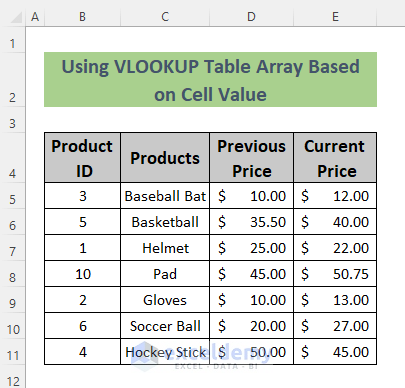
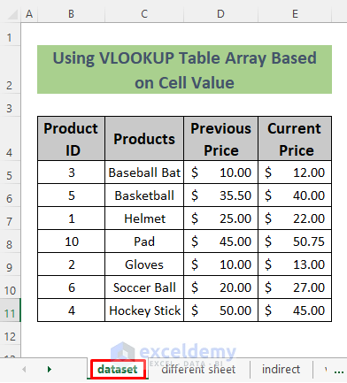
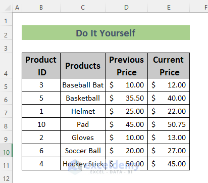
We are using a dataset where we stored some data on sports equipment. We have the Product IDs, Product Names, and their previous and current prices. We’ll extract various values from the table.
How to Make a VLOOKUP Table Array Based on Cell Value in Excel: 5 Simple Ways
Method 1 – Using the Excel VLOOKUP Function to Create a VLOOKUP Table Array Based on Cell Value
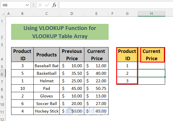
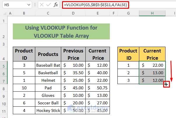
We want to see the Current Prices of the Products that have an ID number less than or equal to 3.
Steps:
- Make two new columns for the chosen Product IDs and their corresponding Current Prices.
- Insert the ID values you want to search.
- Select cell H5 and insert the following formula in it.
=VLOOKUP(G5,$B$5:$E$11,4,FALSE)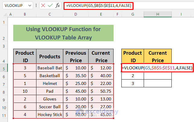
We look up the value in G5 in the B5:E11 table_array. The absolute reference for the table_array avoids the Value not Available Error (#N/A) when copying the formula. We want to see the current price of the products, which are in the 4th column, so we chose 4 as col_index_num. We need an exact match, so we put FALSE for [range_lookup].
- Hit the Enter button and you will see the Current Price of the Product that has the ID number 1 in cell H5.
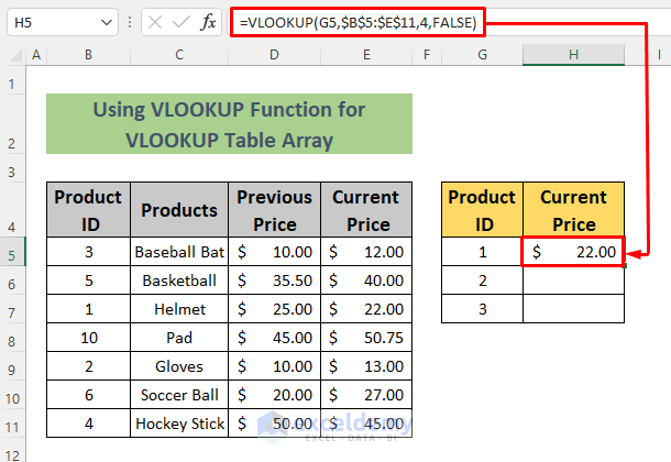
- Use the Fill Handle to AutoFill down.
Read More: How to Expand Table Array in Excel
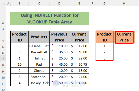
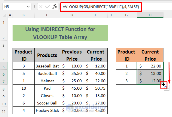
Method 2 – Using the INDIRECT Function to Create a VLOOKUP Table Array Based on Cell Value
Steps:
- Make 2 new columns for the chosen Product IDs and their corresponding Current Prices.
- Insert the IDs you want to search.
- Select cell H5 and insert the following formula in it.
=VLOOKUP(G5,INDIRECT("B5:E11"),4,FALSE)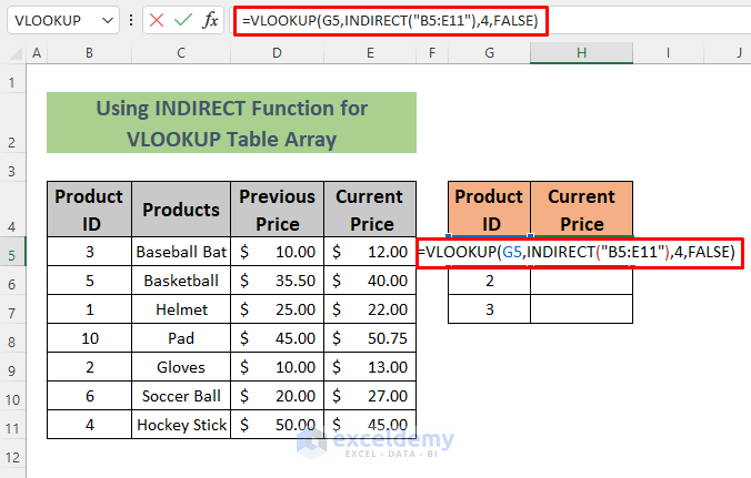
The INDIRECT function makes the range B5:E11 an absolute reference for the table_array.
- Hit the Enter button and you will see the Current Price of the Product that has the ID number 1 in cell H5.
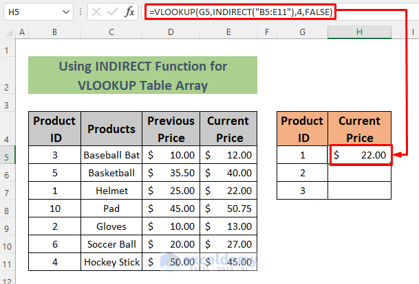
- Use the Fill Handle to AutoFill down.
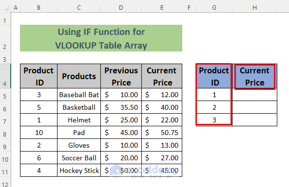
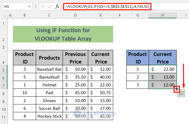
Method 3 – Utilizing the Excel IF Function to Create a VLOOKUP Table Array
Steps:
- Make two new columns for the chosen Product IDs and their corresponding Current Prices.
- Insert the IDs you want to search.
- Select cell H5 and insert the following formula in it.
VLOOKUP(G5,IF(G5<=3,$B$5:$E$11),4,FALSE)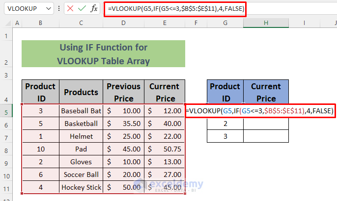
The IF function presents an additional check for the search ID value.
- Hit the Enter button and you will see the Current Price of the Product that has the ID number 1 in cell H5.
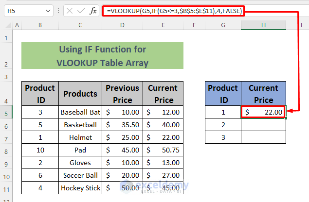
- Use the Fill Handle to AutoFill down.
Read More: How to Name a Table Array in Excel
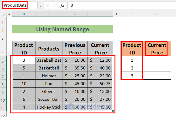
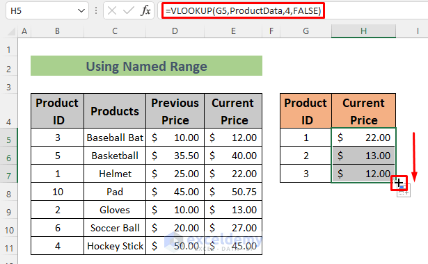
Method 4 – Creating a VLOOKUP Array by Applying a Named Range
Steps:
- Make two new columns for the chosen Product IDs and their corresponding current prices.
- Select the range B5:E11 and give it a name. We chose the name ProductData.
- Select cell H5 and insert the following formula in it.
=VLOOKUP(G5,ProductData,4,FALSE)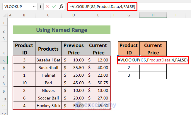
- Hit the Enter button and you will see the Current Price of the Product that has the ID number 1 in cell H5.
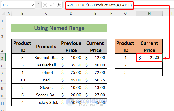
- Use the Fill Handle to AutoFill down.
Method 5 – Using a Table Array in a Different Sheet to Apply VLOOKUP
Steps:
- Make two new columns for the chosen Product IDs and their corresponding previous prices in a new sheet.
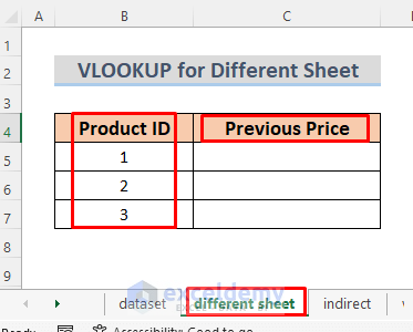
- The lookup array will come from the dataset sheet.
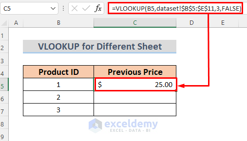
- Select cell C5 and insert the following formula in it.
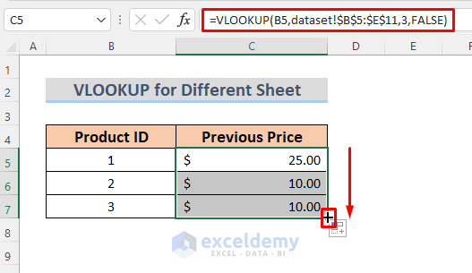
=VLOOKUP(B5,dataset!$B$5:$E$11,3,FALSE)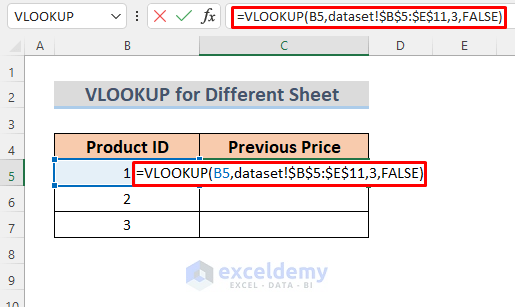
The reference for the lookup array is preceded by the sheet name and an exclamation mark, which indicates it’s in another sheet.
- Hit Enter.
- Use the Fill Handle to AutoFill down.
Practice Section
We have provided a practice section in the download file so you can test these methods.
Download the Practice Workbook
Related Articles
<< Go Back to Table Array in Excel | Excel VLOOKUP Function | Excel Functions | Learn Excel
Get FREE Advanced Excel Exercises with Solutions!
