How to Expand Table Array in Excel (5 Simple Ways)

If you want to expand a table array in Excel, then this article will be helpful for you. The main objective of this article is to explain how to expand table array in Excel.

Download Practice Workbook

5 Simple Ways to Expand Table Array in Excel

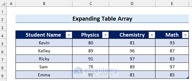
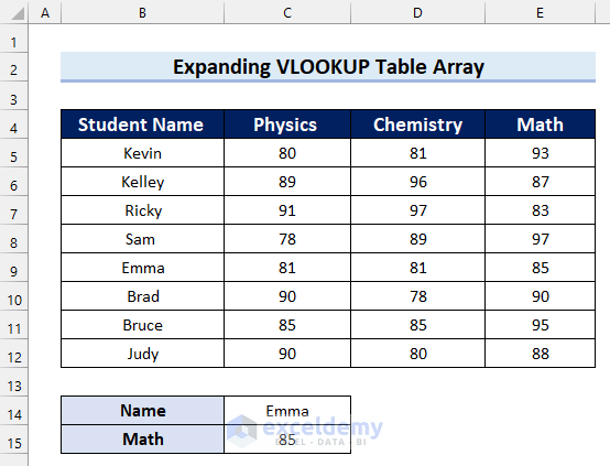
Here, I have taken the following dataset to explain this article. This table contains Student Name and their obtained marks in Physics, Chemistry, and Math. I will use this dataset to explain how to expand table array in Excel.

1. Manually Expanding Table Array by Typing

In this first method, I will explain how to expand table array in Excel manually by typing. Let’s see the steps.

Steps:

To begin with, I will add a new column to my table array.

• Firstly, select the cell where you want your column header. Here, I selected cell F4.
• Secondly, in cell F4 write the name you want for your column header. Here, I wrote English.

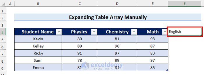
• Thirdly, press ENTER and you will get your new column.

Now, I will add a new row to my table array.

• Firstly, select the cell from where you want to start the new row. Here, I selected cell B10.
• Secondly, in cell B10 type the value you want to show. Here, I wrote Brad because I want to insert obtained marks for a student named Brad.

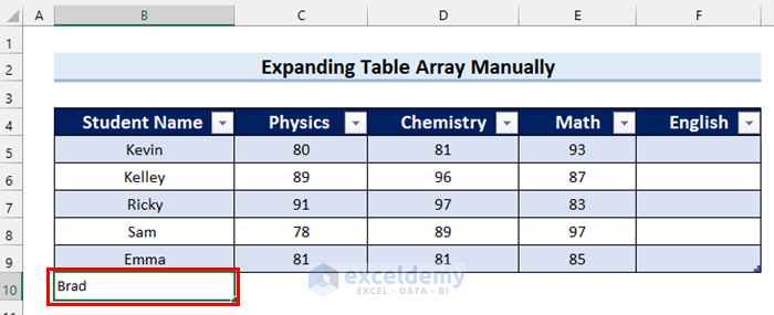
• Thirdly, press ENTER and you will get your row.

Here, you can see that I have gotten a new row for the student named Brad.

Now, I have inserted 2 more rows in the same way to my table array.

Finally, I entered the obtained numbers for every student in each subject and got the expanded table array I wanted.

Read More: How to Edit Table Array in Excel (2 Suitable Ways)

2. Using Insert Command to Expand Table Array in Excel

Here, I will explain how to expand table array in Excel using the Insert command. Let’s see the steps.

Steps:

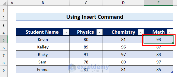
• Firstly, select any cell from the last column of your table array. Here, I selected cell E5.

• Secondly, go to the Home tab from the Ribbon.
• Thirdly, select Insert.
• After that, select Insert Table Columns to the Right.

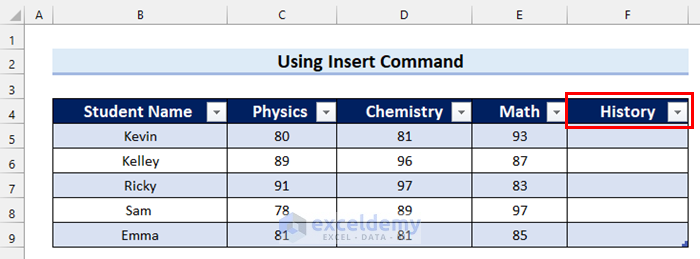
Now, you will see a new column is added to your table array.

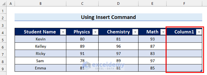
• Next, change the column name as you want. Here, I wrote History as the column header.

Here, I will add new rows to my table array.

• Firstly, select a cell from the last row of your table array. Here, I selected cell B9.
• Secondly, go to the Home tab.
• Thirdly, select Insert.
• After that, select Insert Table Row Below.

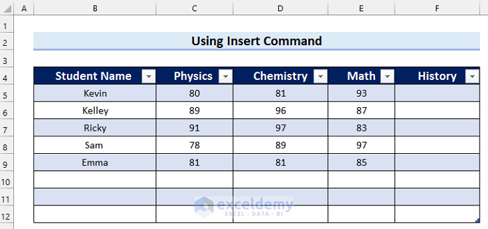
Now, you will see a new row is added to your table array.

Here, in the same way, I added 2 more rows.

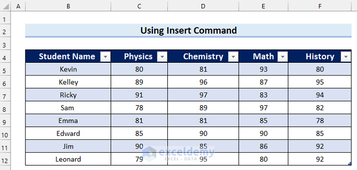
Finally, I have entered the obtained numbers for the added rows and columns and got my desired expanded table array.

Read More: How to Create a Table Array in Excel (3 Methods)

3. Applying Resize Table Feature to Expand Table Array in Excel

In this method, I will explain how you can apply the Resize Table feature to expand table array in Excel. Let’s see the steps.

Steps:

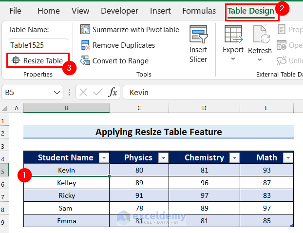
• Firstly, select any cell from your table array.
• Secondly, go to the Table Design tab.
• Thirdly, select Resize Table.

Now, you will see a dialog box named Resize Table has appeared.

• Firstly, select the new table range you want for your expanded table array for Select the new data range for your table.
• Secondly, select OK.

Here, you will see that I have got the expanded table array I wanted.

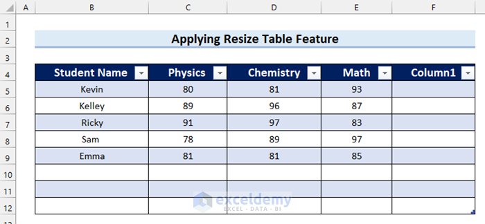
Finally, I entered data in the column and rows I added.

Read More: How to Find Table Array in Excel (4 Suitable Examples)

4. Expanding VLOOKUP Table Array in Excel

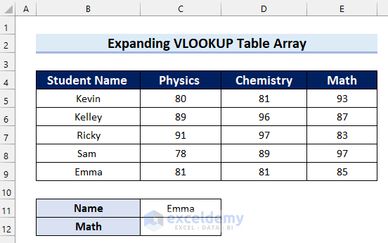
In this method, I will explain how to expand the VLOOKUP table array in Excel. Here, I will show how you can expand the table_array in the VLOOKUP function. In the following image, you can see that I have a dataset. I will find the obtained marks in Math for the student named Emma.

Let’s see the steps.

Steps:

• Firstly, select the cell where you want to find the marks in Math. Here, I selected cell C12.
• Secondly, in cell C12 write the following formula.

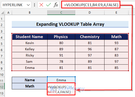
Here, in the VLOOKUP function, I selected cell C11 as lookup_value,  B4:E9 as table_array, 4 as col_index_num, and FALSE as range_lookup because I want an exact match here. The function will return the exact match for the lookup_value.

• Thirdly, press ENTER to get the result.

Here, I have added 3 more rows to my dataset.

Now, you can see the formula is not working after entering a name from the newly added rows. The reason here is that the table_array remains the same.

Now, I will show you how you can expand the table array in a dynamic way.

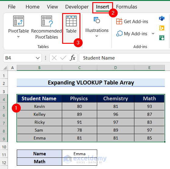
• Firstly, select the data range you want as your table array.
• Secondly, go to the Insert tab.
• Thirdly, select Table.

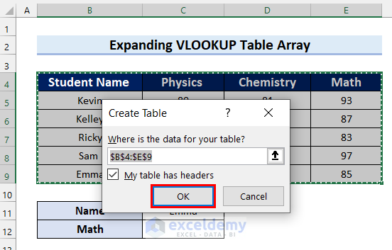
Now, a dialog box named Create Table will appear. The selected range will be inserted automatically here as data for the table.

• After that, select OK.

Here, you can see I have inserted a table.

• Now, select the cell where you want to find the marks in Math. Here, I selected cell C12.
• Next, in cell C12 write the following formula.

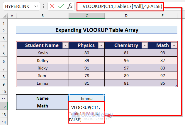
Now, in the VLOOKUP function, I selected cell C11 as lookup_value,  Table17[#All] as table_array, 4 as col_index_num, and FALSE as range_lookup because I want an exact match here. The function will return the exact match for the lookup_value.

• After that, press ENTER.

Here, I have added 3 new rows to the table array.

Now, you can see that the formula works for the values from newly added rows because the table array here is dynamic and can be expanded. This is how you can expand table array for VLOOKUP.

Read More: How to Use VLOOKUP Table Array Based on Cell Value in Excel

5. Using Dynamic Named Range to Expand VLOOKUP Table Array

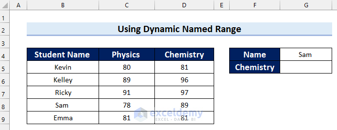
In this method, I will show you how you can expand the VLOOKUP table array in Excel by using Dynamic Named Range. In the following image, you can see my table array. I want to find the obtained marks in Chemistry for Sam using the VLOOKUP function.

Let’s see the steps.

Steps:

• Firstly, select the cell where you want the obtained marks in Chemistry. Here, I selected cell G5.
• Secondly, in cell G5 write the following formula.

Here, in the VLOOKUP function, I selected cell G4 as lookup_value,  B4:D9 as table_array, 3 as col_index_num, and FALSE as range_lookup because I want an exact match here. The function will return the exact match for the lookup_value.

• Thirdly, press ENTER to get the result.

You can see the formula is working.

After that, I added 3 more rows to expand the table array.

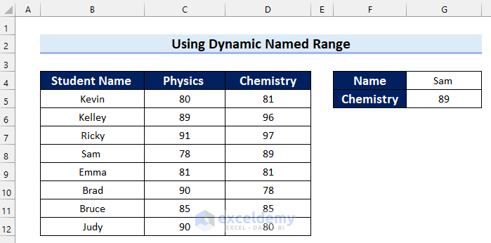
Now, I tried to find obtained marks for a student from the newly added row. You can see that the formula is not working because the table array did not expand as I expanded my dataset.

Here, I will show you how you can make the table array dynamic here. So that, it expands whenever new data is entered.

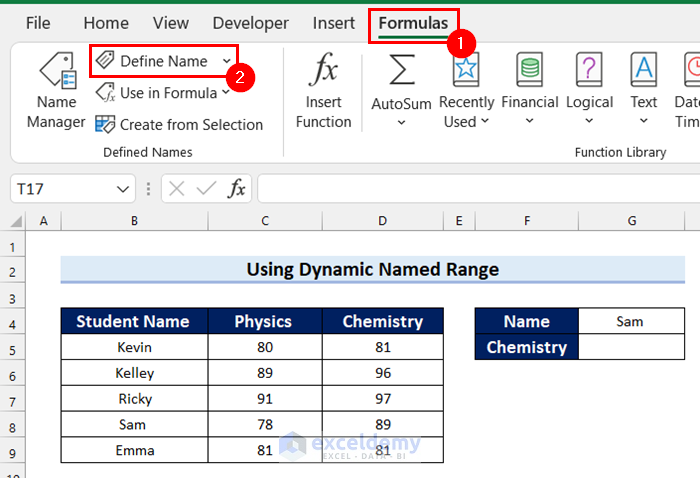
• Firstly, go to the Formulas tab.
• Secondly, select Define Name.

Now, a dialog box will appear.

• Firstly, define the Name. Here, I wrote Dynamic_Range as Name.
• Secondly, write the following formula as Refers to.

• Thirdly, press OK.

• Now, select the cell where you want the obtained marks in Chemistry. Here, I selected cell G5.
• Next, in cell G5 write the following formula.

Here, in the VLOOKUP function, I selected cell G4 as lookup_value,  Dynamic_Range as table_array, 3 as col_index_num, and FALSE as range_lookup because I want an exact match here. The function will return the exact match for the lookup_value.

• Finally, press ENTER.

Now, I have added 3 more rows to expand the table array.

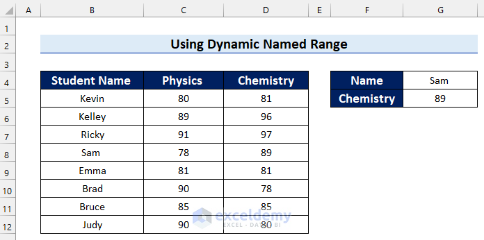
Here, you can see that I used the same formula to find the marks in Chemistry for a student from the newly added rows. And the formula is working. That means I have successfully expanded my table array for VLOOKUP.

Read More: How to Name a Table Array in Excel (With Easy Steps)

Practice Section

Here, I have provided a practice sheet for you to practice how to expand table array in Excel.

Conclusion

To conclude, I tried to cover how to expand table array in Excel. Here, I explained 5 easy and effective ways of doing it.  I hope this article was helpful for you. Lastly, if you have any questions let me know in the comment section below.

Related Articles

• How to Lock Table Array in Excel (2 Effective Ways)
• What Is a Table Array in VLOOKUP? (Explained with Examples)