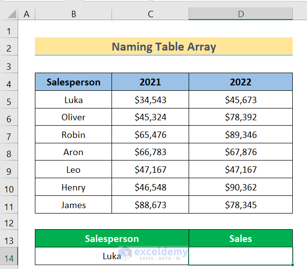
Step 1 – Creating a Table Array
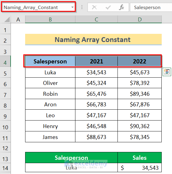
- Arrange the dataset. In this case, we have the Salesperson in Column B and two years, 2021 and 2022, in Columns C and D.
- In cell D14, insert the following formula:
=VLOOKUP(B14,B5:D11,2,0)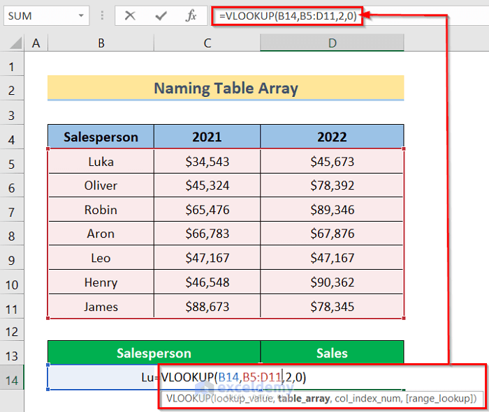
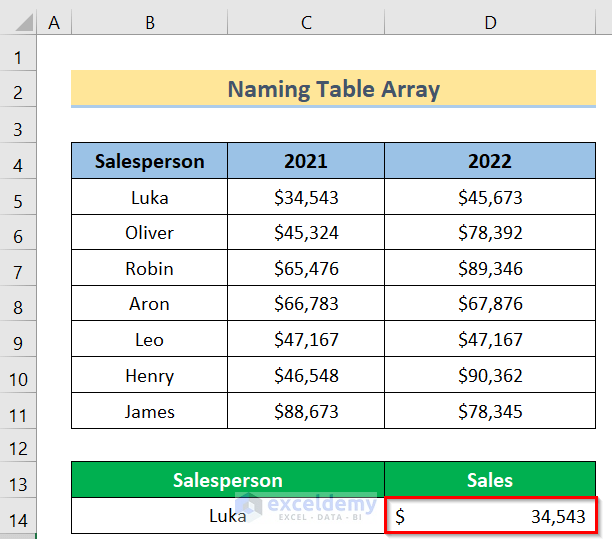
- You will get the desired result.
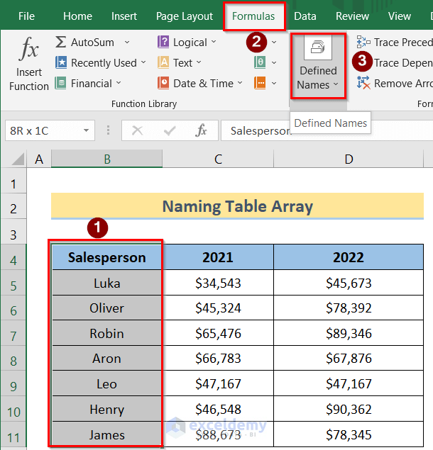
Step 2 – Naming the Table Array
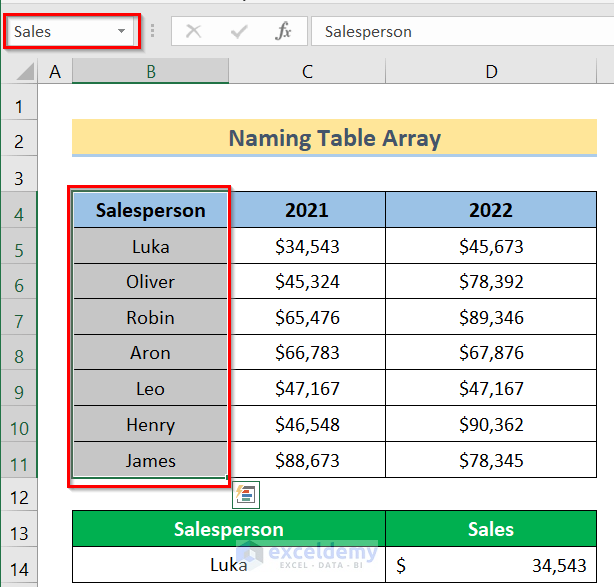
- Select the desired column (in this case Column B).
- Go to Formulas > Defined Names options.
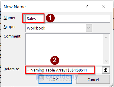
- The New Name dialog box will come on the screen.
- Give a suitable name, select the cells you want to use, and press OK.
- If you write the name, you will get the data like the below image.
Read More: How to Find Table Array in Excel
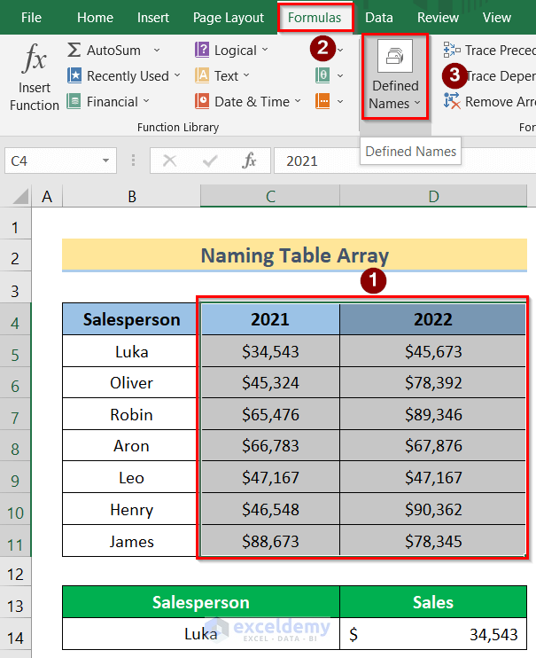
Step 3 – Creating a Dynamic Named Range
- Select a range.
- Go to Formulas > Defined Names.
- In the New Name dialog box, insert the following formula and press OK.
=OFFSET(C5,0,0,COUNTA(C:D),1)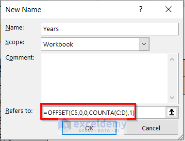
- If you write the name in any cell, you will find the data under this data, like in the previous step.
How Does the Formula Work?
Read More: How to Expand Table Array in Excel
Step 4 – Editing Named Ranges
- Go to Formulas > Defined Names > Name Manager options.
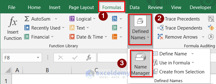
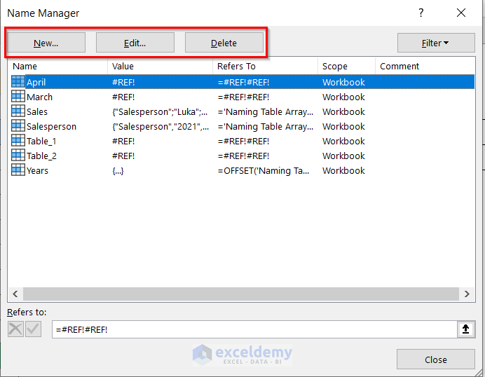
- The Name Manager dialog box will open up on the screen. You can use New, Edit, or Delete according to your need.
- If you want to edit, click the Edit option, and the Edit Name option will appear on your screen. You can make any change in this Name or Refers to options to get the desired result.

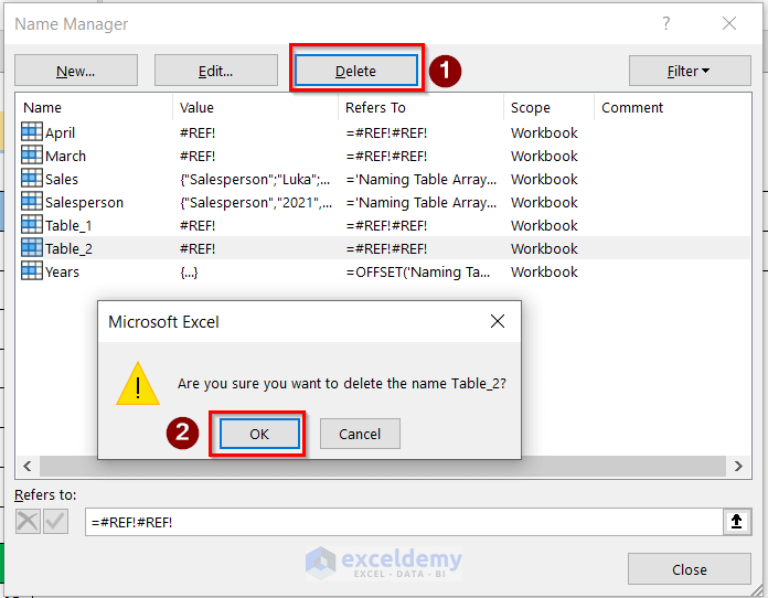
- If you want to delete something, use the Delete option and choose OK, like the image below.
How to Name an Array Constant
Steps:
- Go to Formulas > Defined Names.
- The New Name dialog box will open. Name it as you want and select the desired cells and press OK.
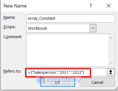
- You will get the desired result.
Download the Practice Workbook
Related Articles
<< Go Back to Table Array in Excel | Excel VLOOKUP Function | Excel Functions | Learn Excel
Get FREE Advanced Excel Exercises with Solutions!
