How to Make VLOOKUP Case Sensitive in Excel?

Consider the following dataset of students. In that dataset, there are two students who have the same first names but different surnames and obtained different scores.

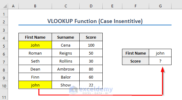
We want to perform a lookup for john’s score. Let’s apply the generic VLOOKUP formula to get the result.

=VLOOKUP(G6,B5:D10,3,0)

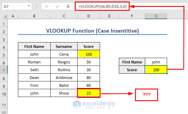
But as you can see in the picture above, it gave us the result of John Cena’s score instead of the score of john Show. It is because VLOOKUP searches for the lookup value in the array and returns the first value that it gets; it doesn’t handle the case sensitivity of letters.

To get a case-sensitive VLOOKUP, you need to execute the function differently.

Method 1 – Using INDEX, MATCH, and EXACT Functions to Make VLOOKUP Case-Sensitive in Excel

The generic formula of the combination of the INDEX and MATCH functions is,

=INDEX(data,MATCH(TRUE,EXACT(value,lookup_column),0),column_number)

Steps:

Click on the cell that you want to have your result value (in our case, the cell was G4).
Insert the following formula:

=INDEX(D5:D10,MATCH(TRUE,EXACT(G6,B5:B10),0))

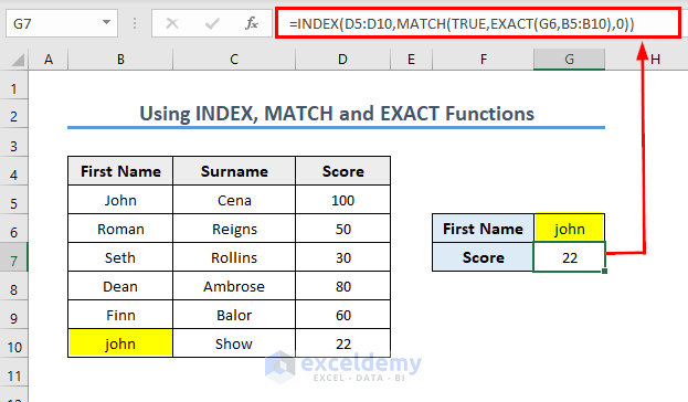
Now, look at the picture above, where you can see that the score of john Show is there, not the score of John Cena.

Formula Breakdown

EXACT(G6,B5:B10) -> The EXACT function in Excel returns TRUE if two strings are exactly the same, and FALSE if two strings don’t match. Here, we are giving the EXACT function an array as a second argument and asking it to find whether the Cell G6 (where we store our lookup value, john) is in there or not. As we have an array as input, we will get an array of TRUE or FALSE in the output. And the output is stored in Excel’s memory, not in a range

Output: {FALSE;FALSE;FALSE;FALSE;FALSE;TRUE}

This is the output of comparing the value of G6 in every cell in the lookup array. As we got a TRUE that means there is an exact match of the lookup value. We just need to find out the position (row number) of that TRUE value in the array.

MATCH(TRUE,EXACT(G6,B5:B10),0) -> become MATCH({FALSE;FALSE;FALSE;FALSE;FALSE;TRUE})

Explanation: The MATCH function returns the position of the first matched value. In this example, we wanted to get an exact match so we set the third argument as 0 (TRUE).

Output: 6

INDEX(D5:D10,MATCH(TRUE,EXACT(G6,B5:B10),0)) -> becomes INDEX(D5:D10,6)

Explanation: The INDEX function takes two arguments and returns a specific value in a one-dimensional range. As we already know the position of the row number (6) that holds our desired value, we are going to use INDEX to extract the value of that position.

Output: 22

Method 2 – Combining Multiple Functions to Make Excel VLOOKUP Case-Sensitive

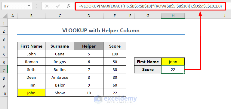
Case 2.1 – Making VLOOKUP Case-Sensitive with a Helper Column

Steps:

Insert a helper column to the left of the column from where you want to fetch the data.
In the helper column, enter the formula “=ROW()“. It will insert the row number in each cell.

=ROW()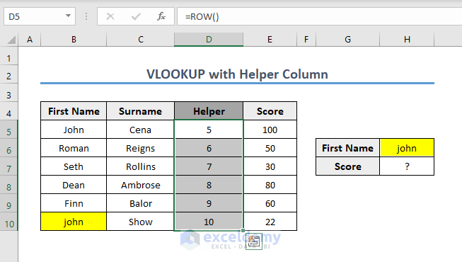

Click on the cell that you want to have your result value (in our case, the cell was H7).
Insert the following:

=VLOOKUP(MAX(EXACT(H6,$B$5:$B$10)*(ROW($B$5:$B$10))),$D$5:$E$10,2,0)

Formula Breakdown

EXACT(H6,$B$5:$B$10) -> EXACT returns an array of TRUE and FALSE values, where TRUE represents case-sensitive matches and FALSE represents the unmatched values. So, in our case, it will return the following array,

Output: {FALSE;FALSE;FALSE;FALSE;FALSE;TRUE}

EXACT(H6,$B$5:$B$10)*(ROW($B$5:$B$10) -> becomes {FALSE;FALSE;FALSE;FALSE;FALSE;TRUE} * {John,Roman,Seth,Dean,Finn,john}

Explanation: It represents the multiplication between the array of TRUE/FALSE and the row number of B5:B10. Whenever there is a TRUE, it extracts the row number. Otherwise, it is FALSE.

Output: {0;0;0;0;0;10}

MAX(EXACT(H6,$B$5:$B$10)*(ROW($B$5:$B$10))) -> becomes MAX(0;0;0;0;0;10)

Explanation: It will return the maximum value from the array of numbers.

Output: 10 (which is also the row number where there is an exact match).

VLOOKUP(MAX(EXACT(H6,$B$5:$B$10)*(ROW($B$5:$B$10))),$D$5:$E$10,2,0) -> becomes VLOOKUP(10,$D$5:$E$10,2,0)

Explanation: It can simply extract the lookup value from the array (D5:D10) and as we want to find an exact match so set the argument 0 (TRUE).

Output: 22

Note: You can insert the helper column anywhere in the dataset. Just make sure to insert it to the left of the column from where you want to fetch the data. You need to adjust the column number in the VLOOKUP function accordingly.

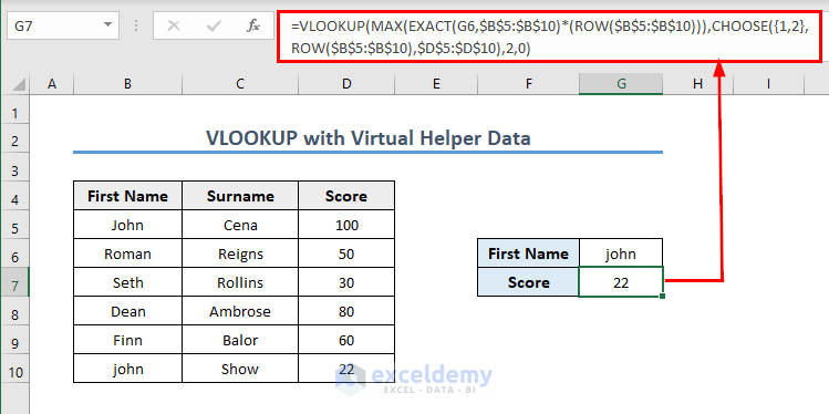
Case 2.2 – Using Virtual Helper Data to Make VLOOKUP Case-Sensitive

Steps:

Click on the cell that you want to have your result value (in our case, the cell was G7).
Insert the following formula:

=VLOOKUP(MAX(EXACT(G6,$B$5:$B$10)*(ROW($B$5:$B$10))),CHOOSE({1,2},ROW($B$5:$B$10),$D$5:$D$10),2,0)

The following part of the full formula works here as the helper data,

=---CHOOSE({1,2},ROW($B$5:$B$10),$D$5:$D$10)---

Formula Breakdown

CHOOSE({1,2},ROW($B$5:$B$10),$D$5:$D$10) -> If you illustrate this formula by selecting it and pressing F9, it will give you the result as,

Output: {5,100;6,50;7,30;8,80;9,60;10,22}

Explanation: It represents an array that shows us the row number and the value associated with it from the given array divided by comma (,). And each semicolon (;) represents the new row number following it. So as it seems like, it created two columns consisting of row number and the column which has the return lookup value (i.e. row number and Score column in our case).

VLOOKUP(MAX(EXACT(G6,$B$5:$B$10)*(ROW($B$5:$B$10))),CHOOSE({1,2},ROW($B$5:$B$10),$D$5:$D$10),2,0 -> becomes VLOOKUP(10,{5,100;6,50;7,30;8,80;9,60;10,22},2,0)

Explanation: When you apply the VLOOKUP function, it simply looks for the lookup value in the first column from the two virtual data columns and returns the corresponding value (i.e. Score). The lookup value here is the combination of the MAX and EXACT functions that we got from the calculation of the above Helper Column discussion.

Output: 22

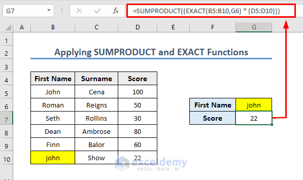
Method 3 – Applying SUMPRODUCT and EXACT Functions to Make VLOOKUP Case-Sensitive in Excel

Generic Formula:

=SUMPRODUCT(- -( EXACT(value,lookup_column)),result_column)

Steps:

Click on the cell that you want to have your result value (in our case, the cell was G4).
Insert the following formula:

=SUMPRODUCT((EXACT(B5:B10,G6) * (D5:D10)))

Formula Breakdown

EXACT(B5:B10,G6) -> EXACT returns an array of TRUE and FALSE values, where TRUE represents case-sensitive matches and FALSE represents the unmatched values. So, in our case, it will return the following array:

Output: {FALSE;FALSE;FALSE;FALSE;FALSE;TRUE}

SUMPRODUCT((EXACT(B5:B10,G6) * (D5:D10))) -> become SUMPRODUCT({FALSE;FALSE;FALSE;FALSE;FALSE;TRUE} * {100,50,30,80,60,22})

Explanation: SUMPRODUCT then simply multiplies the values in each array together to extract a final array, {FALSE;FALSE;FALSE;FALSE;FALSE;22}. And then sum and return the value.

Output: 22

The FALSE values cancel out all the other values. The only values that survive are those that are TRUE.

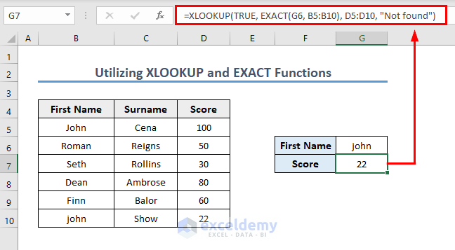
Note: if there are multiple matches in the array, then SUMPRODUCT will return the sum of all those matched values. Also, SUMPRODUCT works only with numeric values, it doesn’t work with text. So, if you want to get a unique text value, then utilize the above methods that we have discussed.

Method 4 – Making VLOOKUP Case-Sensitive with XLOOKUP and EXACT Functions

Generic Formula:

=XLOOKUP(TRUE,EXACT(lookup_value, lookup_array), return_array, “Not Found”)

Steps:

Click on the cell that you want to have your result value (in our case, the cell was G4).
Insert the following formula:

=XLOOKUP(TRUE, EXACT(G6, B5:B10), D5:D10, "Not found")

Formula Breakdown

EXACT(G6, B5:B10) -> EXACT returns an array of TRUE and FALSE values, where TRUE represents case-sensitive matches and FALSE represents the unmatched values. So, in our case, it will return the following array:

Output: {FALSE;FALSE;FALSE;FALSE;FALSE;TRUE}

XLOOKUP(TRUE, EXACT(G6, B5:B10), D5:D10, “Not found”) -> becomes XLOOKUP({FALSE;FALSE;FALSE;FALSE;FALSE;TRUE}, {100,50,30,80,60,22}, “Not found”)

Explanation: XLOOKUP searches the given array (in our case, the array was B5:B10) for the TRUE value and returns a match from the return array (D5:D10).

Output: 22

Remember that, if there are multiple same values in the lookup column (including the letter case), the formula will return the first match.

Note: This XLOOKUP formula will only work in Excel 365.

Key Points to Remember

As the range of the data table array to search for the value is fixed, don’t forget to put the dollar ($) sign in front of the cell reference number of the array table.
When working with array values, don’t forget to press Ctrl + Shift + Enter on your keyboard while extracting results. Pressing only Enter doesn’t work while working with array values unless you work in Excel 365.
After pressing Ctrl + Shift + Enter, you will notice that the formula bar encloses the formula in curly braces {}, declaring it as an array formula. Don’t type those brackets {} yourself, as Excel automatically does this for you.