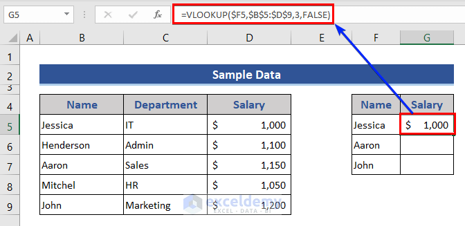
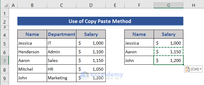
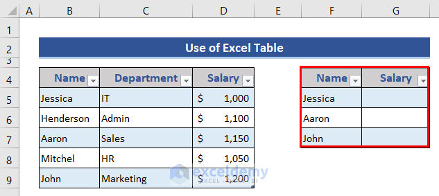
How to Copy VLOOKUP Formula in Excel (7 Easy Methods)

We will consider the following dataset. Here, we applied a VLOOKUP formula on Cell G5. Then, we’ll copy the formula.

Method 1 – The Simple Copy-Paste Method to Copy a VLOOKUP Formula

Steps:

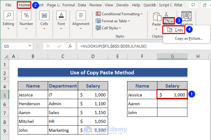
Move to Cell G5.
Click on the Copy option from the Clipboard group from the Home tab.

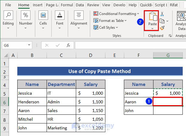
Go to the next cell G6.
Click on the Paste option from the Clipboard group.

Look at the dataset.

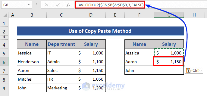
We can see VLOOKUP formula of the corresponding Cell G6 has been pasted.
Copy the formula to Cell G7.

You can also use keyboard shortcuts:

Select cell G5 and press Ctrl + C.
Go to cell G6 and press Ctrl + V.
Paste the formula with Ctrl + V to all necessary cells.

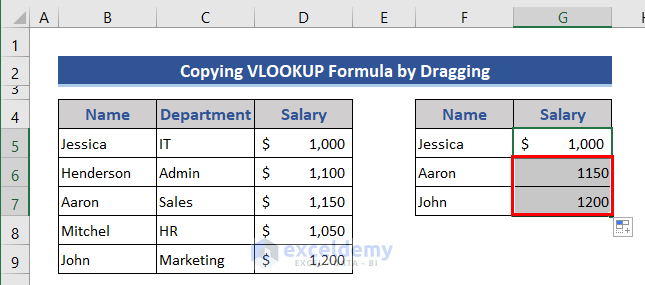
Method 2 – Copy the VLOOKUP Formula Down a Column by Dragging

Steps:

Place the cursor at the bottom-right corner of cell G5.

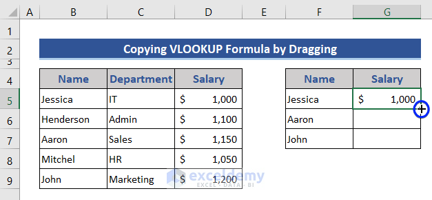
You’ll see a plus symbol (+) there.
Drag this plus symbol down to cell G7.

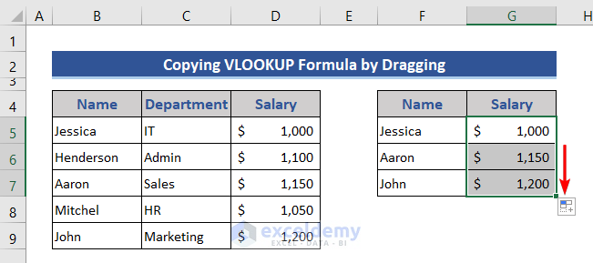
If you don’t need to copy the formatting, click on the down arrow at the right-bottom of Cell G7.

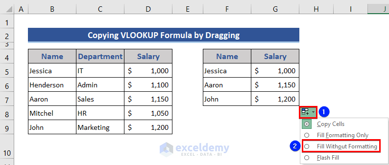
Choose the Fill Without Formatting option.

Method 3 – Copy a VLOOKUP Formula to the Entire Column

Steps:

Hover over the Fill Handle icon for cell G5.

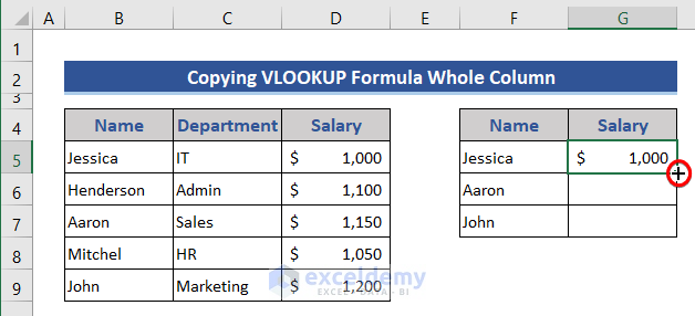
Double-click the Fill Handle icon.

The VLOOKUP formula has been copied through Column G. Like in method 2, we can also remove the formatting from the copied cells.

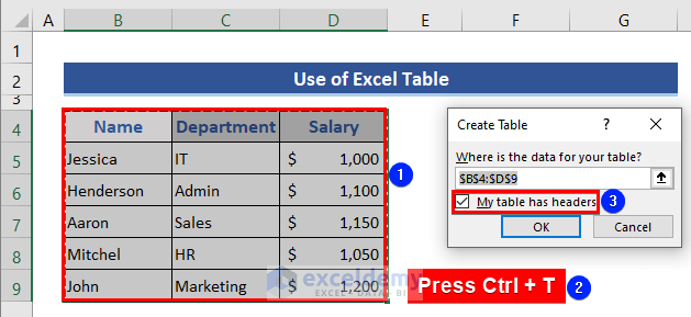
Method 4 – Create an Excel Table to Copy a VLOOKUP Formula

Steps:

Select the Range B5:D9.
Press Ctrl + T.
The Create Table box appears with the selected range.
Check the My table has headers option.
Press the OK button.

We can see a table has been formed.

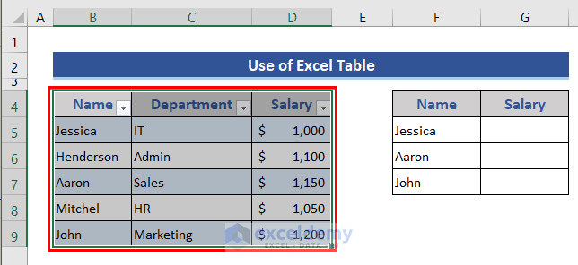
Create another table from the range F5:G7.

Go to Cell G5 and insert the following formula:

=VLOOKUP([@Name],Table1,3,FALSE)

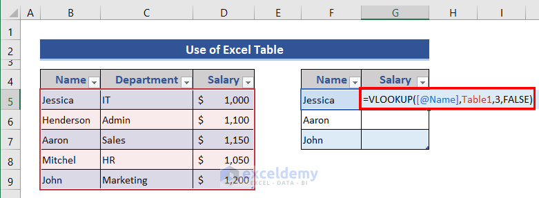
Press the Enter button.

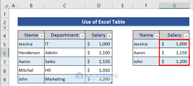
The inserted formula has been copied to all cells of the Salary column of the table.

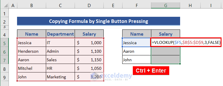
Method 5 – Insert a VLOOKUP Formula in One Cell and Copy to Multiple Cells with a Single Button Press

Steps:

Select Range G5:G9.
Press the F2 button to go to the edit mode.

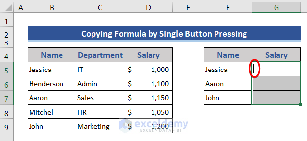
Insert the following formula and press the Ctrl + Enter buttons.

=VLOOKUP($F5,$B$5:$D$9,3,FALSE)

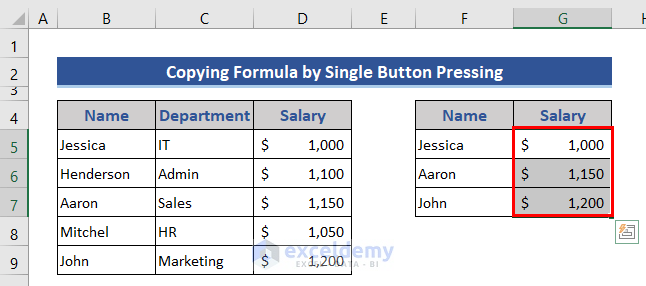
This fills the column with the AutoFilled formula.

Method 6 – Apply a Keyboard Shortcut to Copy VLOOKUP Formula in Excel

Steps:

Place the cursor on Cell G6.
Press Ctrl + D from the keyboard.

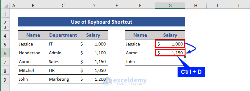
The formula has been copied from cell G5.

The formula will copy only to the next adjacent cell that contains a formula. If the adjacent cell does not contain a formula, this method will not work.

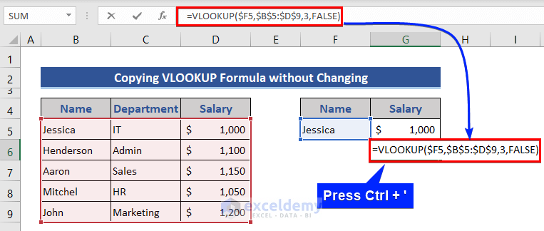
Method 7 – Replicate a VLOOKUP Formula Without Changing Cell Reference

Case 1 – Keyboard Shortcut

Go to the adjacent cell of Cell G5.
Press Ctrl + ‘ (apostrophe) and the Enter button.

Case 2 – Absolute Cell Reference

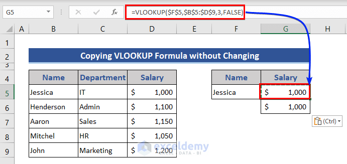
Apply the absolute cell reference in the formula. Look at the formula of Cell G5 in the image for reference.
Copy and paste this formula following any method above.