How to Find Column Index Number in Excel VLOOKUP (2 Ways)

Get FREE Advanced Excel Exercises with Solutions!

We all know that the VLOOKUP function in Excel has 4 arguments. One of them is the col_index_num. i.e. column index number. Finding the column index number is easy, but if you have a long dataset, you might need a way to find it other than just manually searching it. In this article, we will see 2 ways to find Column Index Number in the Excel VLOOKUP function.


Download Practice Workbook

Download this practice workbook to exercise while you are reading this article.


What Is Column Index Number in Excel VLOOKUP Range?

The column index number is a number used in the VLOOKUP formula. This number defines the column of the table array selected for the VLOOKUP operation, that will return after the completion of the operation. This is also called the match column.


2 Methods to Find and Input Column Index Number in Excel VLOOKUP Function

There are two options to find and input column index numbers in the Excel VLOOKUP function. We will discuss those two methods in the below section. Let us have a dataset of people with names, departments, and salaries. We will apply the VLOOKUP operation to get the salary based on names after finding the column index number.

Dataset to find Column Index Number


1. Find and Insert VLOOKUP Column Index Number Manually

In this section, we will find out the column index number and then insert that in the formula manually in the VLOOKUP formula in Excel.

📌 Steps:

  • First, we add two new rows to the dataset.

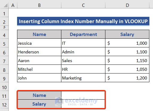
One for name and another one for salary.

  • After that, we input a name in the corresponding box of Name.
  • Then, put the following formula on Cell C12.
=VLOOKUP(C11,B5:D9,3,FALSE)
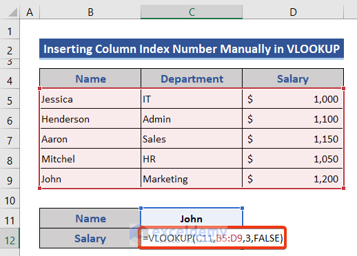
Insert Column Index Number Manually in VLOOKUP function

Here, we selected Range B5:D9, and our resultant column is 3rd of that range. So, we use 3 in the col_index_num section of the VLOOKUP function.

  • Press the Enter button.

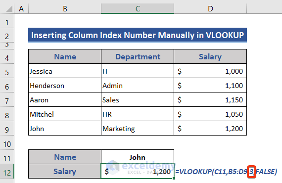
Our VLOOKUP operation is complete after manually inputting the column index number.

Read More: How to Count Columns for VLOOKUP in Excel (2 Methods)


2. Input Column Index Number Inside VLOOKUP With the Help of COLUMN Function

The COLUMN function returns the column number of a reference.

In this section, we will find out the column index number using the COLUMN function. And that result will be used in the VLOOKUP function.

📌 Steps:

  • We move to Cell C12. Then, put the following formula.
=VLOOKUP(C11,B5:D9,COLUMN(D5)-COLUMN(B5)+1,FALSE)
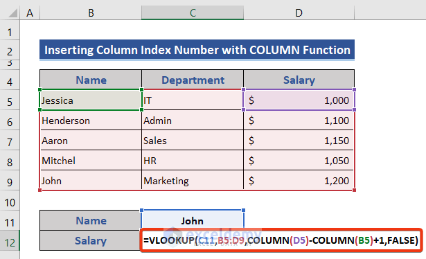
Insert Column Index Number with column function in VLOOKUP function

We can see the COLUMN function is used in the formula. Now, we will subtract the first column number of the table_array from the resultant column number of the VLOOKUP function and lastly add 1.

  • Finally, press the Enter button to see whether the result is accurate or not.
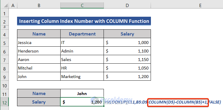
We get the same result. It means the COLUMN function has successfully worked.

Read More: How to Find Column Number Based on Value in Excel


Conclusion

In this article, we described two methods to find out the column index number in Excel and used that in the VLOOKUP function. I hope this will satisfy your needs. Please have a look at our website ExcelDemy and give your suggestions in the comment box.


Related Articles

Alok Paul

Alok Paul

Hello, this is Alok. I am working as an Excel & VBA Content Developer at Exceldemy. I want to provide solutions to various Excel-based problems. I completed my study at East West University major in Telecommunications Engineering. I love traveling, reading books, playing cricket.

We will be happy to hear your thoughts

Leave a reply

Advanced Excel Exercises with Solutions PDF


ExcelDemy
Logo