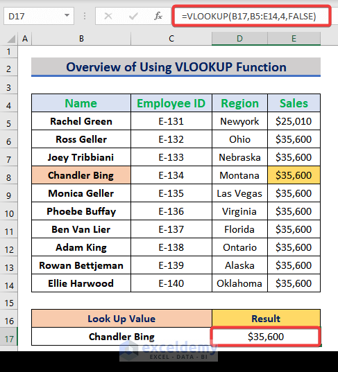
How to Use VLOOKUP Function with Exact Match in Excel

In this article, we’ll describe four examples of how to use the VLOOKUP function with an exact match effectively. Here is the overview of the dataset we’ll use in our examples.

Excel VLOOKUP function exact Match

Introduction to VLOOKUP Function

Syntax:

=VLOOKUP(lookup_value, table_array, col_index_num, [range_lookup]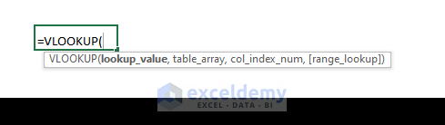

Arguments

Arguments	Required/Optional	Explanation
Lookup_value:	Required	The value in the first column that we want to look up.
Table_array	Required	The table array in which to search for data.
Col_index_num	Required	An integer, the number of the column from the left in which the value to be returned should be found.
[range_lookup]	Optional	Specifies whether the search should return an exact match or not

Notes

If there is no exact match in the data array, we can use TRUE to return an approximate match.

true = approximate match

For an exact match, we use FALSE.

false = exact match

If neither TRUE nor FALSE are specified, the default of TRUE, i.e. approximate match, is applied.

Availability

The VLOOKUP function is available from Excel 2003 onwards. We used Office 365 for this article.

Excel VLOOKUP Function for Exact Match: 4 Practical Examples

Example 1 – Finding a Particular Student’s Marks in a Specific Subject

Suppose we have a dataset of students’ mark sheets. We will use the VLOOKUP function to find particular students’ marks in a subject.

For example, let’s find out what mark, if any, Phoebe Buffays obtained in Mathematics.

Steps:

In cell D17, enter the following formula:

=VLOOKUP(B17,B5:E14,3,FALSE)

Press Enter.

Phoebe Buffay’s mark in Math is returned – 48.

Formula Breakdown

In the VLOOKUP function, B17 is the lookup_value, B5:E14 is the table_array, 3 is the col_index_num, and FALSE is the [range_lookup].
The VLOOKUP function looks up the value of B17 in the table array in the range B5 to E14. As the column index number is 3, the corresponding value of cell B17 from column 3 is returned.

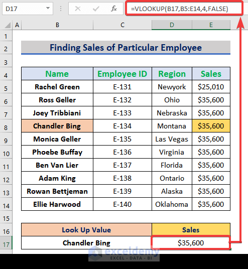
Example 2 – Finding Sales of a Particular Employee

Suppose now we have a dataset of Sales statements of a company which contains the employee’s Name, ID, Region, and Sales. We will use the VLOOKUP function to find particular employees’ sales.

For example, let’s find out Chandler Bings’ sales.

Steps:

In cell D17, insert the following formula:

=VLOOKUP(B17,B5:E14,3,FALSE)

Press Enter.

The sales of Chandler Bings is returned – $35,600.

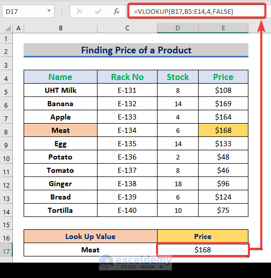
Example 3 – Finding Price of a Particular Product

Suppose we have a dataset of prices of various products in a daily super shop which contains the product’s Name, Rack No, Stock, and Price. We will use the VLOOKUP function to find a particular product’s price.

For example, let’s find out the price of Meat.

Steps:

In cell D17, enter the following formula:

=VLOOKUP(B17,B5:E14,3,FALSE)

Press Enter.

The price of Meat is returned – $168.

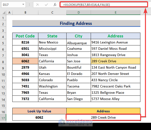
Example 4 – Finding an Address

Suppose we have a dataset of addresses which contains the Postcode, State, City, and Address. We will use the VLOOKUP function to find an Address.

For example, let’s find an Address based on a Postcode.

Steps:

In cell D17, enter the following formula:

=VLOOKUP(B17,B5:E14,3,FALSE)

Press Enter.

The Address matching the Postcode is returned – 289 Creek Drive.

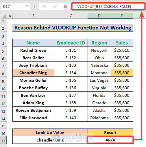
Reason Behind VLOOKUP Function Not Working

Sometimes VLOOKUP function might return an #N/A error instead of the expected result. Some of the possible reasons are:

The formula must contain the correct look_up value. Here, the look_up value cell is B17. Selecting any cell except B17 will cause a #N/A error.
The Table array is not selected properly. It must contain the look_up value. In the picture below, #N/A is displayed because the selected range starts from C5 to E14.
If the Col_index_num is not inserted correctly, it may return #N/A.