Method 1 – Applying the VLOOKUP Function to Search for Specific Text in Excel
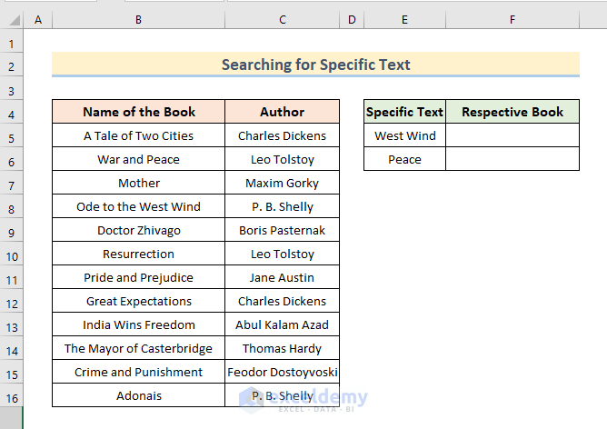
We can use partially matched text to find data from a range of cells in Excel. To demonstrate, I have introduced a dataset containing the Name of the Book and Author, and I will show you how to find a book’s name by inserting a part of it.
Steps:
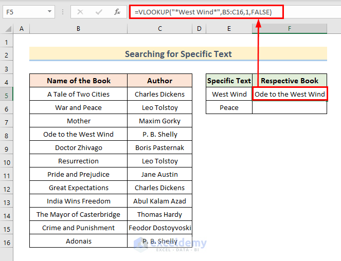
- Enter the following formula in Cell F5.
=VLOOKUP("*West Wind*",B5:C16,1,FALSE)- Press Enter.
- We will now see the Book Name matched with the entry we’ve made using the VLOOKUP function.
In the formula,
- “*West Wind*” is the lookup value.
- B5:C16 is the lookup range.
- 1 denotes the column number in the table to search for.
- False denotes the match should be exact.
- We can also change the lookup value with cell reference.
- To do this, just insert the following formula instead.
=VLOOKUP("*"&E6&"*",B5:C16,1,FALSE)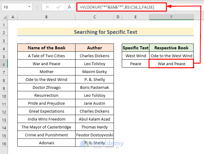
Read More: How to Use VLOOKUP Function with Exact Match in Excel
Method 2 – Using the VLOOKUP Function to Check Presence of Text Value Among Numbers
Steps:
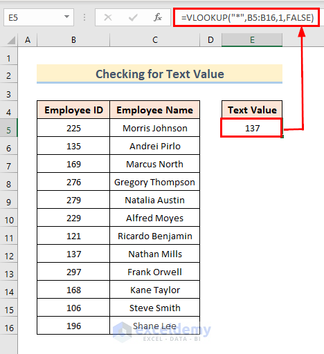
- Enter the following formula in Cell E5.
=VLOOKUP("*",B5:B16,1,FALSE)- Press Enter to see the text value among the numbers.
- In this example 137 was stored as a text value.
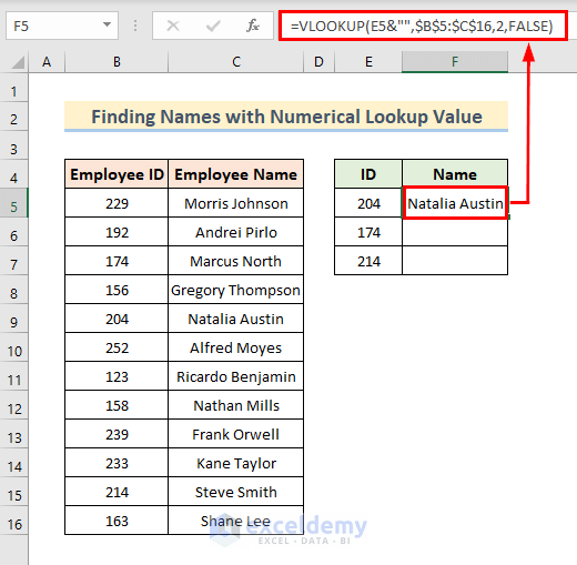
Method 3- Finding Names Using VLOOKUP with Numerical Lookup Value Inserted as Text
In the dataset below we will try and find the Employee Name by using the Employee ID. Here, the Employee IDs are the numerical lookup value but they are stored as texts.
- Enter the following formula in Cell F5.
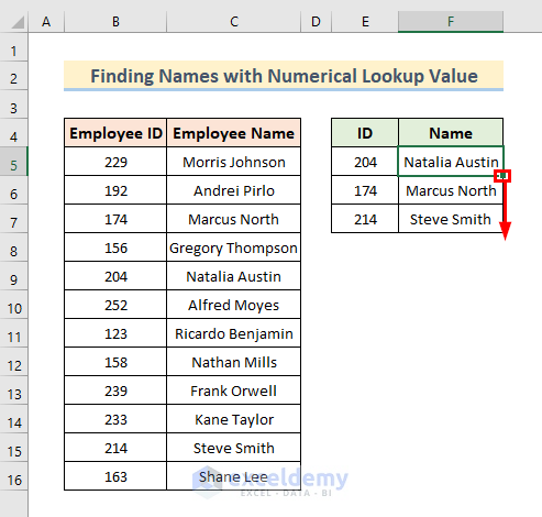
=VLOOKUP(E5&"",$B$5:$C$16,2,FALSE)- Press Enter.
- Use the AutoFill option to see the results for the cells below.
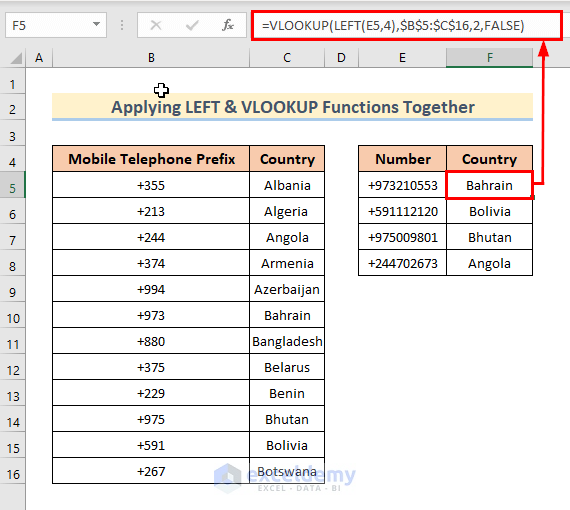
Method – 4. Utilizing the LEFT & RIGHT Functions with VLOOKUP to Find Text
4.1 Apply LEFT and VLOOKUP Functions Together
Steps:
- Enter the following formula in Cell F5.
=VLOOKUP(LEFT(E5,4),$B$4:$C$23,2,FALSE)- Hit Enter.
- Use the Fill Handle to see the results for the cells below.
4.2 Combine RIGHT and VLOOKUP Functions
Steps:
- Enter the following formula in Cell F5.
=VLOOKUP(RIGHT(E5,3),$B$4:$C$23,2,FALSE)- Hit Enter.
- Use the Fill Handle to see the results for the cells below.
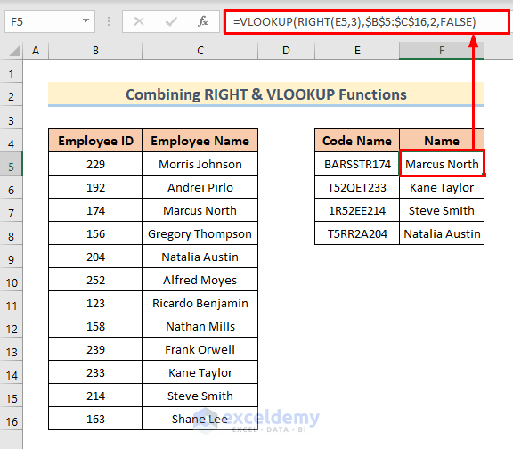
In the formula, the RIGHT function takes 3 right digits from the value of Cell E5 which in turn acts as a lookup value for the VLOOKUP function.
Read More: How to Use VLOOKUP with Two Lookup Values in Excel
A Suitable Alternative to the VLOOKUP Function to Search Text in Excel
Instead of VLOOKUP, we can also use the INDEX & MATCH functions together to search text.
- Enter the following formula in Cell F5.
=INDEX($B$5:$B$16,MATCH("*"&E5&"*",$B$5:$B$16,0))- Press Enter.
- You will see the searched text value instantly.
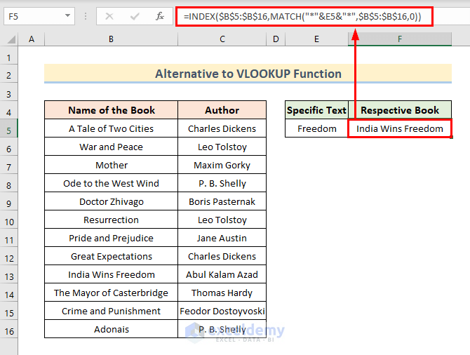
In the formula,
- MATCH(“*”&E5&”*”,$B$5:$B$16,0): gives the row number from $B$5:$B$16 which matches the value from E5.
- The INDEX function takes the output from the MATCH function and finds the text value.
Download Practice Workbook
You can download the practice workbook here.
Further Readings
- How to Apply Double VLOOKUP in Excel
- How to Find Second Match with VLOOKUP in Excel
- VLOOKUP and Return All Matches in Excel
- VLOOKUP Fuzzy Match in Excel
- Excel VLOOKUP to Find Last Value in Column
- How to Apply VLOOKUP by Date in Excel
- Return the Highest Value Using VLOOKUP Function in Excel
- VLOOKUP with Numbers in Excel
<< Go Back to Excel VLOOKUP Function | Excel Functions | Learn Excel
Get FREE Advanced Excel Exercises with Solutions!
