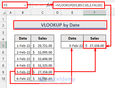
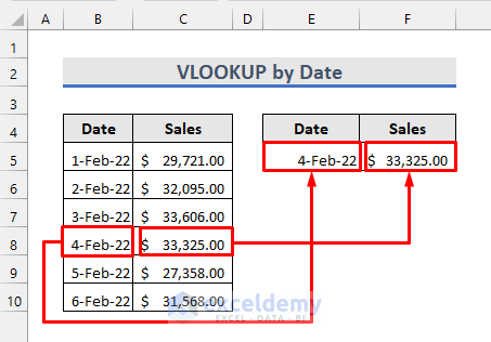
The following picture gives an idea of how VLOOKUP by date works.
Apply VLOOKUP by Date in Excel
We are going to use the following dataset to illustrate how to apply VLOOKUP by date in Excel. The dataset contains the sales amounts corresponding to different dates.
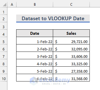
We want to enter the date in cell E5 and find the corresponding amount of sales in cell F5.
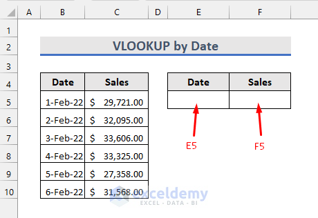
Steps
- Enter the following formula in cell F5:
=VLOOKUP(E5,B5:C10,2,FALSE)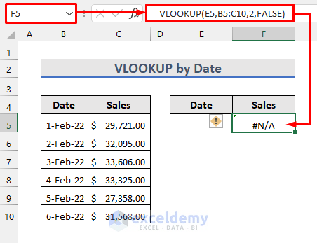
- Enter a date in cell E5 to get the desired sales amount as follows.
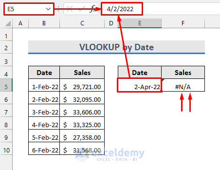
You must enter the date in the same format as in the dataset which is MM/DD/YYYY in this case.

If the date you are looking for doesn’t exist in the dataset, it will show a #N/A error. For example, enter 2/4/2022 instead of 2/4/2022 and you will see the following.
How does the Formula Work?
The VLOOKUP function consists of the following arguments:
VLOOKUP(lookup_value, table_array, col_index_num, [range_lookup])It asks for the value to lookup(lookup_value). Then the range of data to look up(table_array). After that, it asks the column number(col_num_index) where the return value exists in that range. Finally, the range_lookup argument asks whether you want to look for an Approximate Match(TRUE) or an Exact Match(FALSE).
If we compare this with the formula entered in cell F5 then we get,
- Lookup_value = E5 which contains the date we look for.
- Table_array = B5:C10 which contains the dataset.
- Col_index_num = 2 which is the second column of the dataset containing the sales amounts we wanted to find out.
- Range_lookup = FALSE, meaning looking for an exact match.
Read More: How to Use VLOOKUP Function with Exact Match in Excel
Perform VLOOKUP to Return a Date in Excel
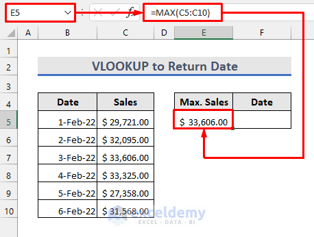
We want to find the date corresponding to the maximum sales amount.
Steps
- Enter the following formula in cell E5:
=MAX(C5:C10)The MAX function in this formula will return the maximum sales amount from the Sales column.
- Enter the following formula in cell F5:
=VLOOKUP(E5,B5:C10,1,FALSE)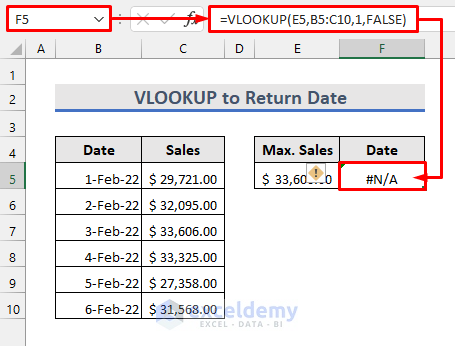
We get an error because VLOOKUP only looks from left to right.
- Swap the Date and the Sales columns.
- Change the formula in cell E5 to the following:
=MAX(B5:B10)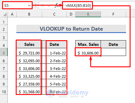
- Apply the following formula in cell F5:
=(VLOOKUP(E5,B5:C10,2,FALSE)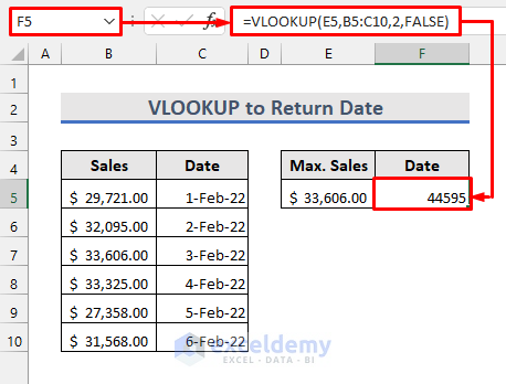
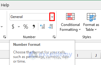
- Change the date format of that cell from the Home tab.
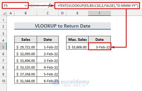
- An alternative is to apply the following formula instead of the earlier one in cell F5.
=TEXT(VLOOKUP(E5,B5:C10,2,FALSE),"D-MMM-YY")The TEXT function in this formula will change the value obtained from the VLOOKUP formula to the date format.
Read More: How to Use VLOOKUP to Search Text in Excel
Things to Remember
- You must enter dates in the same format as the dates in the dataset.
- The lookup value must be in a column earlier than the column which contains the return value.
- Make sure the text format is inside double quotes (“”) in the TEXT function.
Download the Practice Workbook
Related Articles
- How to Use VLOOKUP with Two Lookup Values in Excel
- How to Apply Double VLOOKUP in Excel?
- How to Find Second Match with VLOOKUP in Excel
- VLOOKUP and Return All Matches in Excel
- VLOOKUP Fuzzy Match in Excel
- Excel VLOOKUP to Find Last Value in Column
- Return the Highest Value Using VLOOKUP Function in Excel
- VLOOKUP with Numbers in Excel
<< Go Back to VLOOKUP a Range | Excel VLOOKUP Function | Excel Functions | Learn Excel
Get FREE Advanced Excel Exercises with Solutions!
