How to Use VLOOKUP to Find Duplicates in Two Columns

In this tutorial, I am going to show you 8 quick tricks to use VLOOKUP to find duplicates in two columns. You can quickly use these methods even in large datasets to find duplicate data values. Throughout this tutorial, you will also learn some important excel tools and functions which will be very useful in any excel related task.

Download Practice Workbook

You can download the practice workbook from here.

8 Quick Tricks to Use VLOOKUP to Find Duplicates in Two Columns

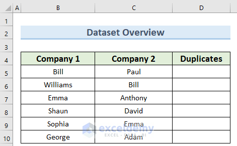
We have taken a concise dataset to explain the steps clearly. The dataset has approximately 6 rows and 3 columns. Initially, we are keeping all the cells in General format. For all the datasets, we have 3 unique columns which are Company 1, Company 2, and Duplicates. Although we may vary the number of columns later on if that is needed.

1. Using VLOOKUP With #N/A Error to Find Duplicates

The VLOOKUP function in Excel gives us the option to look up vertically in a data table. In this first method, we will use this function only to find duplicates in two columns.

Steps:

• First, go to cell D5 and insert the following formula:

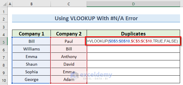
Here, the formula is looking for the values of the Company 2 column in the Company 1 column. FALSE means we do not need range lookup.

• Now, press Enter and this will display the duplicate data in column D with a #N/A error when no match exists.

So this was the first method to achieve what we were looking for.

Read More: INDEX MATCH vs VLOOKUP Function (9 Practical Examples)

2. Utilizing VLOOKUP With IFERROR To Find Duplicates in Two Columns

The IFERROR function in excel allows us to show a custom result whenever there is an error. We will use this function with the VLOOKUP function to find duplicates in two columns of data.

Steps:

• To begin with, double-click on cell D5 and enter the below formula:

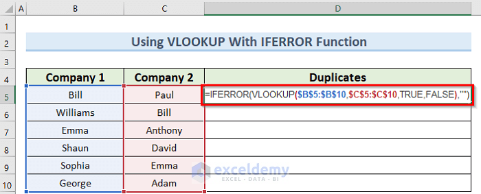
Here, VLOOKUP($B$5:$B$10,$C$5:$C$10,TRUE,FALSE) gives the value as Bill. If it returns any error then we get an empty string.

• Next, press the Enter key and you should get the common names from the two companies with empty spaces for no match case.

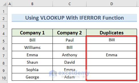
In this way, you can quickly look for duplicate values in any dataset.

Read More: 10 Best Practices with VLOOKUP in Excel

3. Using VLOOKUP and IFNA Functions

The IFNA function in excel can spot a #N/A error and give a particular result in that case. Let us see how to use VLOOKUP to find duplicates in two columns with this function.

Steps:

• To begin this method, double-click on cell D5 and insert the formula below:

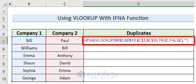
In this formula, if the VLOOKUP formula gives any #N/A error, then we get an empty string. Otherwise, we get the value.

• Next, press the Enter key and consequently, this will find the duplicate employee names within the two companies as in the image below.

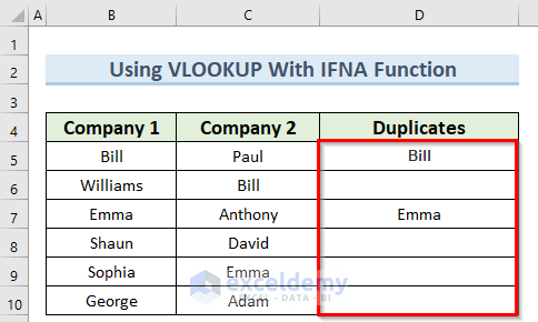
As you can see, the IFNA function gives an easy option to find duplicates.

Read More: How to Use IF ISNA Function with VLOOKUP in Excel

4. Find Duplicates by VLOOKUP and ISERROR Functions

The ISERROR function in Excel checks for any sort of error inside a cell. We can perform VLOOKUP to find duplicates in two columns with the help of this function.

Steps:

• To start this method, navigate to cell D5 and type in the following formula:

Here, if there is an error, we get an empty string and for other cases, we get the value as duplicate.

• After that, press the Enter key or click on any blank cell.
• Immediately, this will give you the word Duplicate for the values that exist in both companies.

So this is how we can use this function with VLOOKUP.

Read More: How to Vlookup with Multiple Matches in Excel (with Easy Steps)

Similar Readings

• VLOOKUP Not Working (8 Reasons & Solutions)
• Excel LOOKUP vs VLOOKUP: With 3 Examples
• Use VLOOKUP with Multiple Criteria in Excel (6 Methods + Alternatives)
• How to VLOOKUP and SUM Across Multiple Sheets in Excel
• Excel VLOOKUP to Find Last Value in Column (with Alternatives)

5. Applying VLOOKUP With ISNA Function

The ISNA function also tests a cell value but only for a #N/A error. In the below steps, we will see how to easily apply this function with VLOOKUP to find duplicates in two columns.

Steps:

• As previously, insert the below formula inside cell D5:

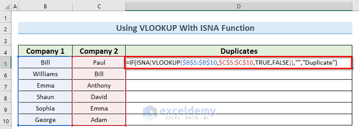
Here, the ISNA function gives a TRUE value for which we get an empty string.

• Finally, press the Enter key and we should get the Duplicate indicator after the formula has performed the VLOOKUP operation.

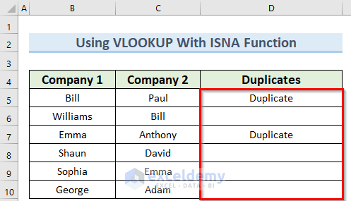
The above method is actually very effective in finding duplicate names within the dataset.

Read More: VLOOKUP and Return All Matches in Excel (7 Ways)

6. Matching Duplicates Values Using IF and MATCH Functions

In this simple method, we will learn to use the IF and MATCH functions to do VLOOKUP to find duplicates in two columns.

Steps:

• First, go to cell D5 and insert the following formula:

Here, the MATCH function returns 2 which is greater than 0. So we get the value of cell B5.

• Next, press Enter and immediately this will look for the duplicate employee names within the two columns and give a #N/A error where it finds no duplicates.

So try this MATCH function to quickly catch duplicates in your data.

7. Using ISNUMBER and MATCH Functions

The ISNUMBER function in excel mainly checks whether a cell contains a numeric value. We will use this function in VLOOKUP to find duplicates in two columns.

Steps:

• At first, navigate to cell D5 and type in the formula below:

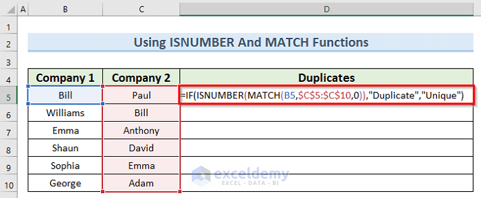
Here, the MATCH function returns a number so the IF function gives the value as Duplicate.

• After that, press the Enter key as before and this will give either a Duplicate or Unique value indicator for all the data values in Company 1 as in the image below.

As we see, you can quickly find copy values using the ISNUMBER function.

8. Finding Duplicates in Different Sheets

For this last method, we will see a unique case where we might need to find duplicates in two columns using VLOOKUP.

Steps:

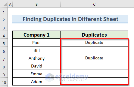
• To begin with this method, navigate to cell D5 and insert the following formula:

Here, the formula is referencing the sheet List 1 and if there is a #N/A error, we get an empty string as before.

• After that, just press the Enter key to confirm or click on any empty cell and this should mark the duplicate values in column C.

In this way, you can find duplicate cell values from multiple sheets.

Conclusion

I hope that you were able to apply the methods that I showed in this tutorial on how to use VLOOKUP to find duplicates in two columns. As you can see, there are quite a few ways to achieve this. So wisely choose the method that suits your situation best. If you get stuck in any of the steps, I recommend going through them a few times to clear up any confusion. Lastly, to learn more excel techniques, follow our ExcelDemy website. If you have any queries, please let me know in the comments.

Further Readings

• How to VLOOKUP and Return Multiple Values Vertically in Excel
• VLOOKUP to Return Multiple Columns in Excel (4 Examples)
• Why VLOOKUP Returns #N/A When Match Exists (with Solutions)
• VLOOKUP with Numbers in Excel (4 Examples)
• How to Use LARGE Function with VLOOKUP Function in Excel
• VLOOKUP Example Between Two Sheets in Excel
• How to Use VLOOKUP to Find Partial Text from a Single Cell