This is an overview.
The ISNA Function in Excel
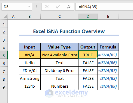
The ISNA function is an INFORMATION function in Excel. It checks whether a cell contains the #N/A error and returns TRUE or FALSE.
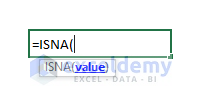
Syntax:
Arguments:
| Argument | Required/Optional | Explanation |
|---|---|---|
| value | Required | A value or expression to be checked for the #N/A! error |
Example 1 – Find the #N/A Error using the ISNA Function
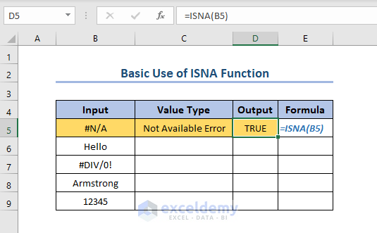
This is the sample dataset.
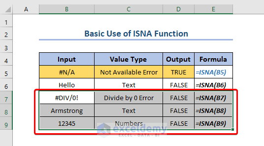
#N/A is displayed in B5. In the Output column (D), the ISNA function is used to check whether data in B5 is available. As data is Not Available (#N/A), the function returns the answer to the question (is the data in a cell available?) as TRUE.
In the second row, there is Text data, in B6.
The ISNA function is used to see if data in B6 is available. The result is FALSE because “Hello” is a text value.
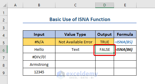
In the other cells the Output is also FALSE.
Example 2 – Using the ISNA with the VLOOKUP and the IF Functions
This is the sample dataset.
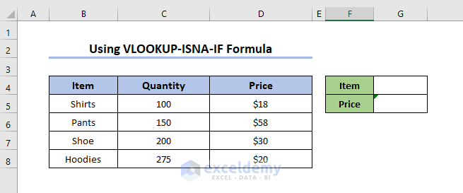
To set the item as the lookup criteria and find the price:
- Enter the formula:
=VLOOKUP(G4,B5:D8,2,0)Here,
- G4 is the lookup value,
- B5:D8 is the lookup_range,
- 2 is the column number
- 0 is used for an exact match.
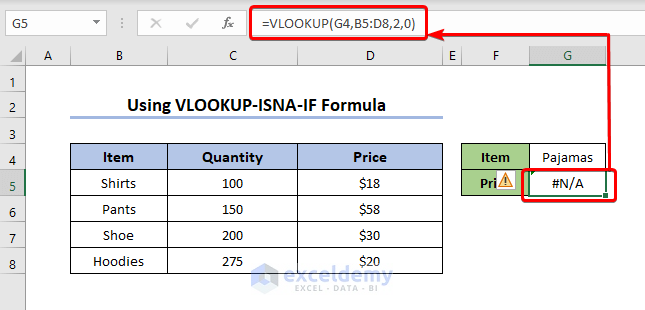
If the lookup value is unlisted, here Pajamas:
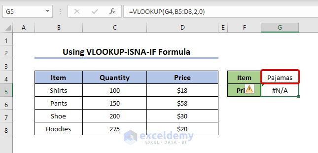
The formula returns #N/A .
- Use the following formula.
=IF(ISNA(VLOOKUP(G7,B5:C8,2,0)),"Not Available",VLOOKUP(G7,B5:C8,2,0))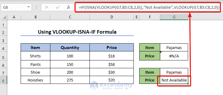
It checks whether the VLOOKUP produced #N/A, using the ISNA Function. It is set to display “Not Available”. Otherwise, it performs the VLOOKUP operation.
Instead of #N/A, “Not Available” is displayed.
Important Note:
You can also use the XLOOKUP function.
Read More: How to Use IF with ISNA Function in Excel
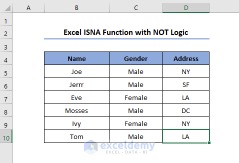
Example 3 – Using the ISNA Function with the NOT Logic
The dataset showcases students’ name, gender and address.
- To find the number of male students whose address is not in NY (New York) and SF (San Francisco), use the formula:
=SUMPRODUCT((C5:C10=C12)*ISNA(MATCH(D5:D10,C13:D13,0)))The MATCH function compares the values and returns them as an array in the ISNA Function. #N/A, is TRUE.
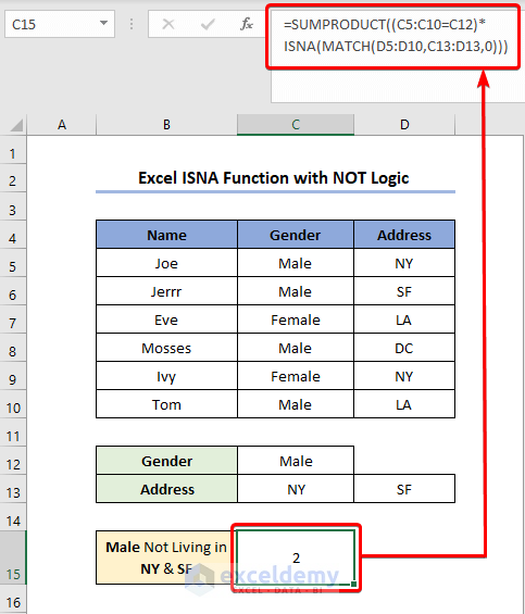
It checks the gender and returns the value in an array. These two arrays are multiplied and another array is found. The SUMPRODUCT function adds the arrays and returns the final output:
2 male students are not from NY or SF.
Things to Remember
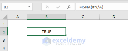
You can insert #N/A directly into the function.
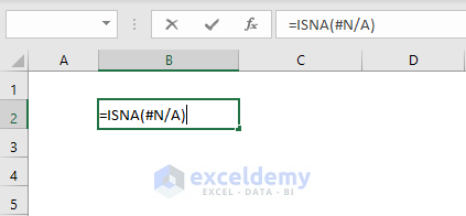
It will return TRUE.
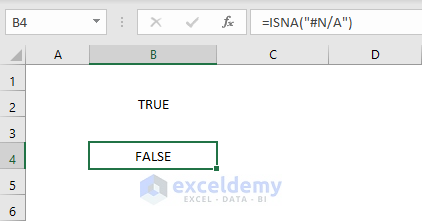
Remember not to enter #N/A within double quotes.
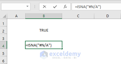
If so, it will be counted as a text string and the function will return FALSE.
Download Practice Workbook
Download the practice workbook.
<< Go Back to Excel Functions | Learn Excel
Get FREE Advanced Excel Exercises with Solutions!
