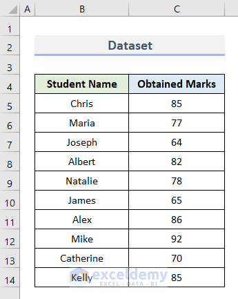
The dataset shows 10 Student Names with their Obtained Marks in an exam.
As a long dataset, find the marks that the student Albert obtained in the exam.Use any type of function that works with lookup value. Use the VLOOKUP function and get the output with this formula.
=VLOOKUP(F4,B5:C14,2,0)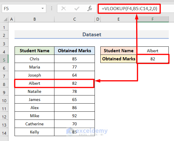
Insert the name Pamela, the output returns a #N/A error as the name is not available in the dataset.
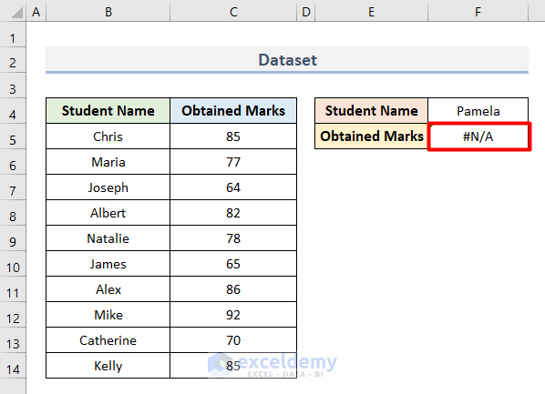
We need to use the IF and ISNA functions to replace this error.
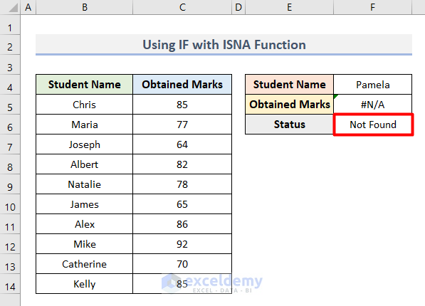
Method 1 – Use IF with ISNA Function to Replace Error in Excel
- Select Cell F6.
- Put this formula inside the cell.
=IF(ISNA(F5),"Not Found", "Found")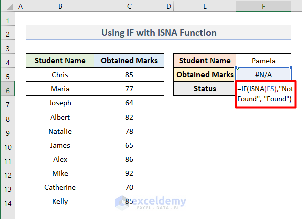
- Press Enter.
- Get the result as Not Found instead of a #N/A error.
Method 2 – Combine IF and ISNA with VLOOKUP Function in Same Table
- Apply this formula in Cell F6.
=IF(ISNA(VLOOKUP(F4, $B$5:$C$14, 2, FALSE)), "Not Found", VLOOKUP(F4, $B$5:$C$14, 2, FALSE))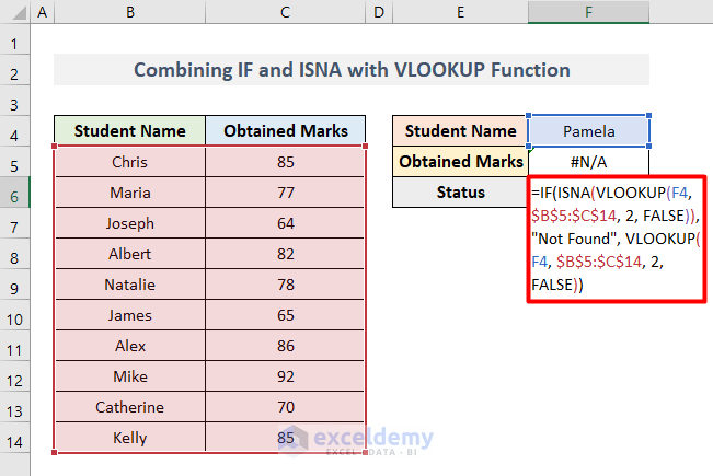
- Hit on Enter.
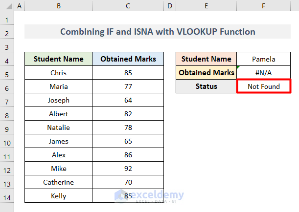
- Get the output as text rather than as a #N/A error.
The VLOOKUP function looks for the lookup value of Cell F4 from the range B5:C14. The function returns a value from column number 2, otherwise FALSE when not found. The IF function runs a logical test based on the ISNA function.
Method 3 – Apply IF and ISNA with MATCH Function for Logical Test in Excel
- Select Cell F6 and insert this formula.
=IF(ISNA(MATCH(F4,$B$5:$C$14,0)), "Not Found", "Found")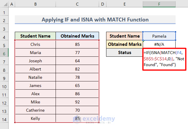
- Press Enter and you will get the following output.
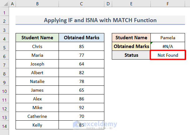
The MATCH function finds and matches the lookup value of Cell F4 from the range B5:C14. Then, we typed 0 for an Exact Match. The IF function runs a logical test based on the ISNA function.
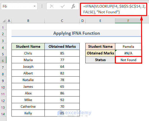
Excel IFNA Function: An Alternative to ISNA-IF Combination
The ISNA function with the IFNA function. Because both of them are applied to check for #N/A error and return TRUE or FALSE. But the major difference is, we need to nest the ISNA and VLOOKUP (or MATCH/any LOOKUP function) functions with the IF function to get the output. The IFNA function directly works without any nested function. The following image shows the output with the IFNA function.
Download Practice Workbook
Get this sample file practice by yourself.
<< Go Back to Excel ISNA Function | Excel Functions | Learn Excel
Get FREE Advanced Excel Exercises with Solutions!

