Excel IFNA function is primarily used to handle the #N/A errors. It returns a specific value as per your instruction if such a #N/A error occurs; otherwise, it returns the absolute value of the function. In this article, we’ve discussed Excel IFNA function in detail with 6 suitable examples.
We will be using the following product price list as our demo dataset to explain all the examples regarding the IFNA function. Now let’s have an overview of our article:
For conducting the session, I will use Microsoft 365 version.
Introduction to Excel IFNA Function
- Function Objective
The IFNA function is used to tackle the #N/A error.
- Syntax
IFNA(value, value_if_na)

- Arguments Explanation
| Argument | Required/Optional | Explanation |
|---|---|---|
| value | Required | Value is to check for the @N/A error. |
| value_if_na | Required | Value to return only if the #N/A error is found. |
- Return Parameter
Value of the first argument or an alternative text.
How to Use Excel IFNA Function: 5 Suitable Examples
In this section, we will show you some easy and simple examples to clarify the concept of this IFNA function. So, you can implement the IFNA function to make your work easier. Let’s see the examples below.
1. Basic Usage of the IFNA Function in Excel
In this example, we will show you the very basic usage of the IFNA function.
So if there’s any valid value available in the value field, then that value will appear as a function output. Otherwise, the value_if_na field will return its specified value as a function output.
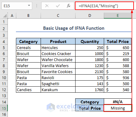
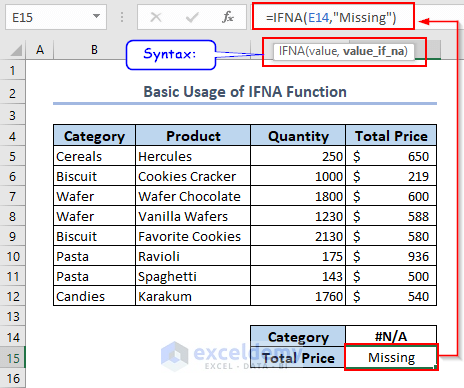
In the above image, there’s already #N/A within cell E14. So if we refer to cell E14 within the value field of the IFNA function, then the value specified in the value_if_na field will appear in cell E15.
- Now insert the formula within cell E15,
=IFNA(E14,"Missing")As we press the ENTER button, we can see the Missing message appear within cell E15 as predicted.
2. Usage of IFNA Function with VLOOKUP Function to Return a Meaningful Massage
First of all, we want to describe the usability of the IFNA function with the VLOOKUP function. This is the most common usage of the IFNA function.
You may want to use the VLOOKUP function to extract values based on a lookup value. Now what’s the inconvenient thing about this VLOOKUP function? It has a complex syntax, as well as, it requires a bundle of rules to follow to work properly.
So by any means, if you do any of the mistakes, then the VLOOKUP will show the #N/A error. Which is nothing but an error that represents, “value is not available”.
Now, suppose you don’t want to allow the #N/A message throughout your dataset. But we’re interested in showing a more meaningful message.
In that case, you can use the IFNA function along with the VLOOKUP function to tackle the error message in a better way.
2.1 Using IFNA Function with VLOOKUP Function in Single Sheet
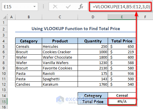
Let’s say for any #N/A error message, we want to show “Missing”. In the image below, we can see the #N/A message within cell E15.
- The formula within cell E15 is:
=VLOOKUP(E14,B5:E12,3,0)If we look closely at the data table below, we can see that the lookup value is Cereal. But there is no such value in the first column of the data table. As a result, #N/A error is showing there.
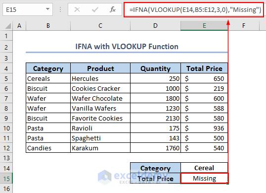
Now if we want to show Missing in replace of #N/A, then we have to use the following formula with the IFNA function.
=IFNA(VLOOKUP(E14,B5:E12,3,0),"Missing")This is how we can use the IFNA function along with the VLOOKUP function.
Formula Breakdown
- Here, E14 stores the lookup value; B5:E12 is the table lookup array; 3 denotes column index; 0 specifies the exact match.
- So, VLOOKUP(E14,B5:E12,3,0) —> look for Cereal and return its corresponding price.
- Output: #N/A. (As there is no category named “Cereal”)
- IFNA(#N/A,”Missing”) —> returns Missing within cell E15 as the value is an error.
2.2 Apply IFNA and VLOOKUP Functions to Search Multiple Findings
Here, we will search for the prices of multiple products at once.
- So, first, write the product’s names. Here, we have written it in D15:D17 cells.
- Then use the following formula in the E15 cell.
=IFNA(VLOOKUP(D15:D17,C5:E12,3,0),"Missing")- Press ENTER and get all of their prices.
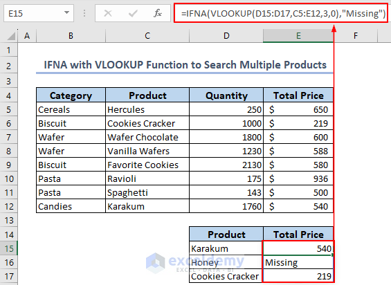
Formula Breakdown
- The VLOOKUP function will search for the value of D15:D17 within the table array of C5:E12. 3 and 0 respectively denoting the column index, and the exact match.
- If there are any unmatched products then the IFNA function will return Missing for them.
2.3 Use IFNA Function with VLOOKUP Function Within Multiple Sheets
Suppose you need to use the VLOOKUP function within multiple sheets. In this case, if there is no similar lookup value in the dataset then you will get an error as output. So, we will combine the IFNA function with the VLOOKUP function to search items across multiple sheets.
First, we will make a list of all products and then apply Data Validation to find the price of a product from that list.

- Make the list for all products.
- Click E7 cell >> from Data tab >> under Data Tools group >> from Data Validation >> select Data Validation.
As a result, you will see the dialog box named “Data Validation”.
- In that dialog box >> select List in the Allow box >> set the reference of all products in the Source box >> press OK.
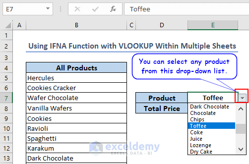
So, you will see a drop-down list beside the E7 cell and can select any product from this drop-down list.
- Now enter the following formula in the E8 cell.
=IFNA(VLOOKUP(E7,'List-1'!B5:E12,3,0),IFNA(VLOOKUP('IFNA-MultipleSheets'!E7,'List-2'!B5:E10,3,0),IFNA(VLOOKUP('IFNA-MultipleSheets'!E7,'List-3'!B5:E11,3,0),"Missing")))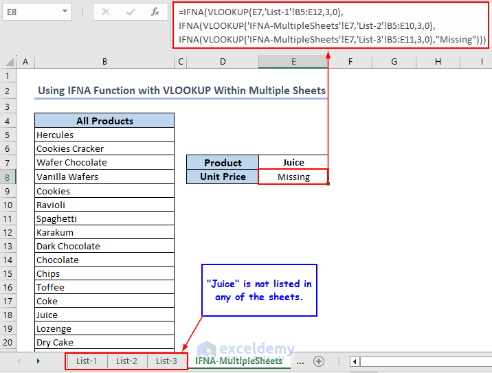
- Then you will get the unit price of the selected product in the E7 cell. As I have selected Juice in the E7 cell which is not listed in any of the sheets, I get “Missing” as output.
Formula Breakdown
- Here, the name of the current worksheet is IFNA-MultipleSheets.
- VLOOKUP(E7,’List-1′!B5:E12,3,0)—> Here look up value is the E7 cell value from the active worksheet. Then the table array is the range B5:E11 from the worksheet named List-1. 3 is the column index, and 0 is for the exact match.
- So, when the VLOOKUP function will not find an exact match from the List-1 worksheet, it will give a null error. Then the IFNA function will go to the 2nd IFNA function.
- The 2nd IFNA function will search for the value of this: VLOOKUP(‘IFNA-MultipleSheets’!E7,’List-2′!B5:E10,3,0). Where the VLOOKUP function will go to the sheet named List-2.
- If the VLOOKUP function still doesn’t get a value then again it will give the null error. This error will affect another IFNA function.
- Lastly, the 3rd VLOOKUP function will search for the E7 cell value from the List-3 worksheet. If still there is no such value then the IFNA function will return Missing.
- As we are using the IFNA function, whenever it will find a value through the VLOOKUP function, then the formula will stop there and give that particular value.
3. Catch #NA Error Using IFNA Function with MATCH Function
While you are using the MATCH function, you can also get a meaningful answer instead of getting the #NA error.
Here, we want to find the row index of a defined product. If the product name doesn’t exist then we want to show “No matched product” in the place of the row index.
- Use the corresponding formula in the E15 cell and press ENTER to get the result.
=IFNA(4+MATCH(D14,C5:C12,0),"No matched product")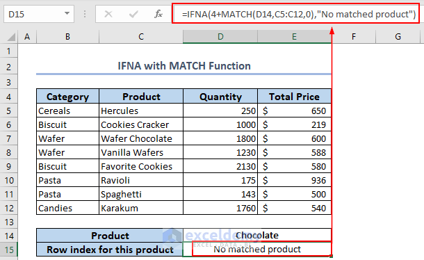
Formula Breakdown
- MATCH(D14,C5:C12,0)—> This MATCH function will search exactly for the cell value of D14 within the range C5:C12.
- Output: #N/A.
- 4+#N/A returns another #N/A.
- So, IFNA(#N/A,”No matched product”)—> gives No matched product.
4. Apply IFNA with INDEX-MATCH Functions to Suppress #NA Error
Here is another example of the application of the IFNA function. You can use the IFNA function with the combination of INDEX, and MATCH functions to make the #NA error understandable.
- In cell D15, enter the following formula. See the result.
=IFNA(INDEX(E5:E12,MATCH(D14,C5:C12,0)),"There is no product like this")
Formula Breakdown
- MATCH(D14,C5:C12,0)—> This MATCH function will search exactly for the cell value of D14 within the range C5:C12.
- Output: #N/A. Which will act as the row number of the INDEX function.
- So, INDEX(E5:E12,#N/A)—> here this INDEX function will return the value from the range E5:E12 according to the mentioned row number. As the row number is a #N/A error, so the INDEX function will also return #N/A error.
- Lastly, IFNA(#N/A,”There is no product like this”) will return “There is no product like this”.
5. Use of IFNA Function to Solve a Mathematical Problem in Excel
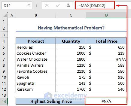
Suppose you want to solve an easy mathematical problem like finding the highest value or calculating a summation. But mistakenly, there is a #N/A error in your dataset. Then you will find another #N/A error after doing that mathematical problem.
See the below image, you will get my point. It is so irritating that a single #N/A error becomes the barrier to doing a tiny calculation.
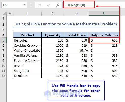
- To solve the problem, create a new column E >> paste the following formula in the E5 cell.
=IFNA(D5,0)- Use the Fill Handle icon to copy the same formula for other cells of the E column. As a result, you will get a 0 instead of the #N/A error.
- Now do your needed calculation with the data of the E column. Like below, I have used the MAX function and got the highest selling price among them.
=MAX(E5:E12)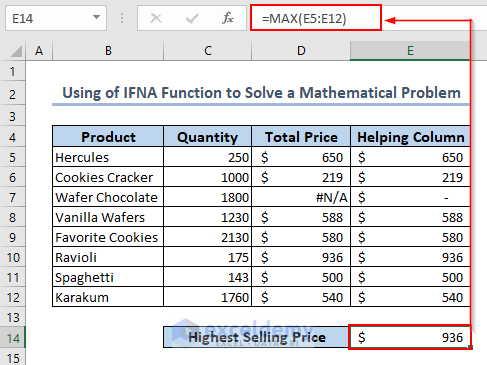
IFERROR Vs IFNA Function in Excel
The IFERROR function handles a wide range of errors whereas the IFNA function tackles only the #N/A i.e. not available error.
For instance, if there’s any typo in your formulas then Excel may return the #NAME error. In this case, the IFERROR function can handle the error by showing an alternating text in replace of the #NAME message.
On the other hand, the IFNA function cares only about the #N/A error. This can display an alternative text in replacing the #N/A error showing.
So, if you want to handle only the #N/A error, then it’s the best practice to use the IFNA function in lieu of the IFERROR function. For the other types of errors, you can use the IFERROR function.
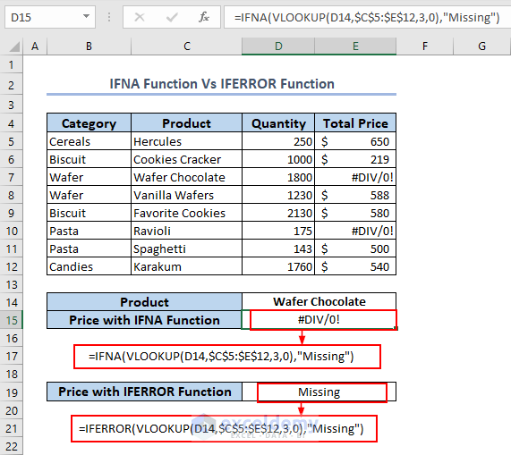
See the above image, there is a division error (#DIV/0!) in our dataset. The IFNA function can’t respond to this error, whereas the IFERROR function can!
Things to Remember
📌 If a cell is empty, then it’s treated as an empty string (“”) but not as an error.
📌 If you don’t fill up the value_if_na field, then the IFNA function will consider this field as an empty string value (“”).
Frequently Asked Questions
1. Which versions of Excel have the IFNA function?
From the version of Excel 2013 to the earlier versions, you will get this IFNA function.
2. Is false and 0 the same in Excel?
Yes, we can use 0 instead of FALSE in any function of Excel.
3. How do you check if a cell is null or empty in Excel?
You can use the ISBLANK function to find the empty cells. This function will return TRUE to the empty cells.
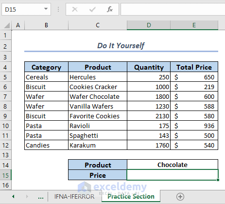
Practice Section
Now, you can practice the explained method by yourself.
Download Practice Workbook
You are recommended to download the Excel file and practice along with it.
Conclusion
To sum up, we have discussed every possible aspect with corresponding examples regarding the Excel IFNA function. You are recommended to download the practice workbook attached along with this article and practice all the methods with that. And don’t hesitate to ask any questions in the comment section below. We will try to respond to all the relevant queries asap.
<< Go Back to Excel Functions | Learn Excel
Get FREE Advanced Excel Exercises with Solutions!

hello Mrinmoy Roy , hope you’re fine…
I hope you can help me…
pls i am trying to make an index formula on excel with different arguments and below is my formula
=INDEX(TABLES!E98:T189, MATCH(1, ($C$3=”TABLES!$D$97:$S$97″) * ($C$4=”TABLES!$C$98:$C$189″) * ($C$5=”TABLES!$B$98:$B$189″) * ($C$6=”TABLES!$A$99:$A$189″), 0))
but i am getting either #value or #N/A error msg . and i can’t figure out why .
my tables are from a different sheet but with same values and the error is in C3 C4 C5 and C6
can you know whay might be the problem ?
Hello Vera,
Thanks for reaching out! Here, in your formula I can see few issues. First, your formula has double quotes around the table references in conditions. These quotes are not necessary; you should directly compare the values. Please check that the cell references in your conditions (C3, C4, C5, C6) contain the correct values that you’re searching for in the specified ranges in the TABLES sheet. Also make sure that the data types match. If one of the values is a text string, the comparison should be done with text.
Here, I am adding the modified formula, try this. If it doesn’t work, please share the Excel file with us!
=INDEX(TABLES!E98:T189, MATCH(1, (TABLES!$D$97:$S$97=$C$3) * (TABLES!$C$98:$C$189=$C$4) * (TABLES!$B$98:$B$189=$C$5) * (TABLES!$A$99:$A$189=$C$6), 0))