Introduction to the VLOOKUP Function

- Function Objective:
The VLOOKUP function is used to look for a given value in the leftmost column of a given table and then returns a value in the same row from a specified column.
- Syntax:
=VLOOKUP(lookup_value, table_array, col_index, [range_lookup])
- Arguments Explanation:
| Argument | Required/Optional | Explanation |
|---|---|---|
| lookup_value | Required | The value which it looks for is in the leftmost column of the given table. Can be a single value or an array of values. |
| table_array | Required | The table in which it looks for the lookup_value in the leftmost column. |
| col_index_num | Required | The number of the column in the table from which a value is to be returned. |
| [range_lookup] | Optional | Tells whether an exact or partial match of the lookup_value is required. 0 for an exact match, 1 for a partial match. The default is 1 (partial match). |
- Return Parameter:
Returns the value of the same row from the specified column of the given table, where the value in the leftmost column matches the lookup_value.
Practices with VLOOKUP in Excel: 10 Best Examples
Part 1 – Beginner Examples and Practices with VLOOKUP
Example 1 – VLOOKUP to Find Specific Data or Array Horizontally from a Table
In the following table, a number of sales data has been recorded for the salesman. We’re going to get the sales record of Peter from the table.
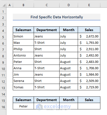
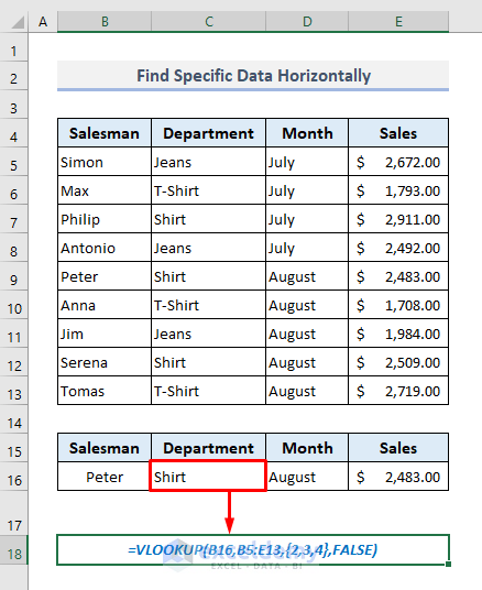
In the output Cell C16, the required formula will be:
=VLOOKUP(B16,B5:E13,{2,3,4},FALSE)After pressing Enter, you’ll get the department, month, and sales value in a horizontal array at once. In this function, we have defined the column index of three Columns C, D, and E in an array of {2,3,4}.
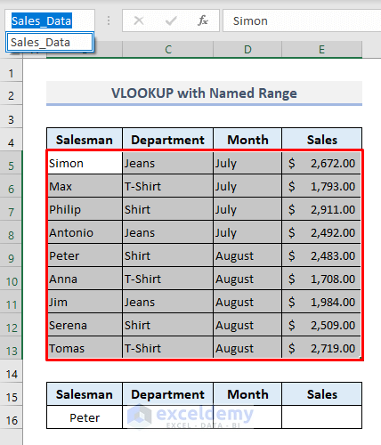
Example 2 – VLOOKUP with a Named Range in Excel
We can define the array or table data with a named range.
- Select the array and then edit the name in the Name Box situated on the left-top corner of the spreadsheet.
- The formula used in the previous example will look like this with the defined named range:
=VLOOKUP(B16,Sales_Data,{2,3,4},FALSE)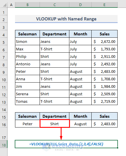
Read More: How to Make VLOOKUP Case Sensitive in Excel
Example 3 – Categorizing Data with VLOOKUP in Excel
We have added an extra column named Category outside the data table or array. We’ll categorize the departments with A, B, or C based on the second table at the bottom.
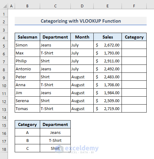
Steps:
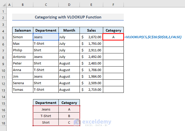
- Select Cell F5 and insert:
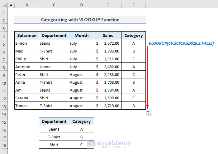
=VLOOKUP(C5,$C$16:$D$18,2,FALSE)- Press Enter.
- Use the Fill Handle to autofill the entire Column F.
Part 2 – Intermediate Examples and Practices with VLOOKUP
Example 1 – Showing an Error Message If Data Wasn’t Found with VLOOKUP
We’re going to find the sales record of Robert, but this name is not available in the Salesman column. We’ll use the IFERROR function here to define a message that will be displayed when the function is unable to match the given criterion.
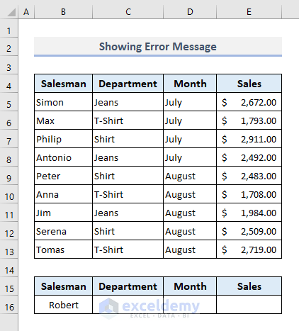
- In Cell C16, the required formula with IFERROR and VLOOKUP functions will be:
=IFERROR(VLOOKUP(B16,Sales_Data,{2,3,4},FALSE),"Not Found")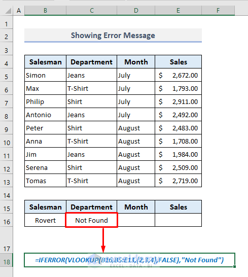
Example 2 – VLOOKUP a Value Containing Extra Space(s)
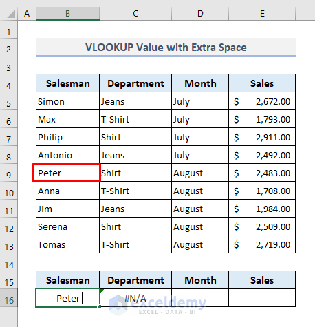
Our lookup value might contain a hidden space sometimes. In that case, our lookup value cannot be matched with the corresponding names present in Column B. So, the function will return an error as shown in the following picture.
To avoid this error message and remove space before starting to look for the specified value, we have to use the TRIM function inside. The TRIM function trims the unnecessary space from the lookup value.
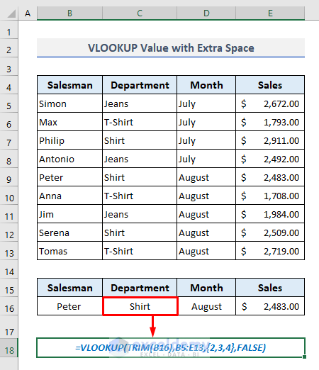
- Since Cell B16 contains an extra space at the end of the name- Peter, the required formula to look for the name Peter only without any space in the output Cell C16 will be:
=VLOOKUP(TRIM(B16),B5:E13,{2,3,4},FALSE)- After pressing Enter, you’ll find the extracted data for Peter.
Related Content: How to Use Dynamic VLOOKUP in Excel
Example 3 – VLOOKUP with MATCH Function in Excel
We’ll find the Department (check value in C17) for Antonio (criteria in C16).
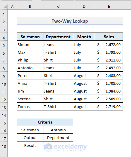
- In the output Cell C18, the required formula will be:
=VLOOKUP(C16,B4:E13,MATCH(C17,B4:E4,0),FALSE)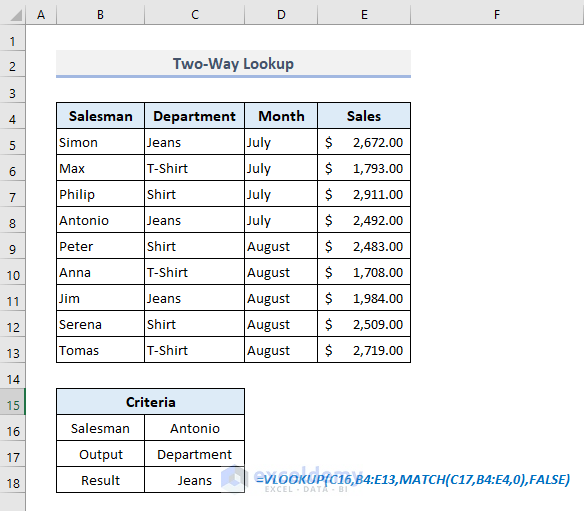
You can change the values of the cells in C16 and C17 to other salesmen and different column headers you need to search by, respectively.
Example 4 – Pulling Data Based on a Partial Match with VLOOKUP
We’ll look for the actual name with a partial text “ton” (listed in B16) and extract the sales record for that salesman.
- The required formula in Cell C16 should be:
=VLOOKUP("*ton*",B5:E13,{2,3,4},FALSE)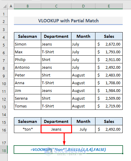
Example 4 – Extracting the Last Value in a List with VLOOKUP
Extracting the last or final value in a long range of cells is too simple with the VLOOKUP function.
Column B contains numbers with random values. We’ll extract the last value from this column or the range of cells B5:B14.
- The necessary formula with the VLOOKUP function in the output Cell D8 will be:
=VLOOKUP(9.99999999999999E+307,$B$5:$B$14,TRUE)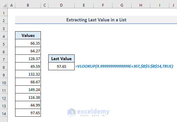
How Does the Formula Work?
- In this function, the lookup value is a huge number that has to be searched in the range of cells B5:B14.
- The lookup criteria here in the third argument is TRUE which denotes the approximate match of that number.
- The VLOOKUP function looks for this huge value and returns the last value based on the approximate match as the function is unable to find the defined number in the column. Since the function goes through the entire range, it will get the last value.
Part 3 – Advanced Examples and Practices with VLOOKUP
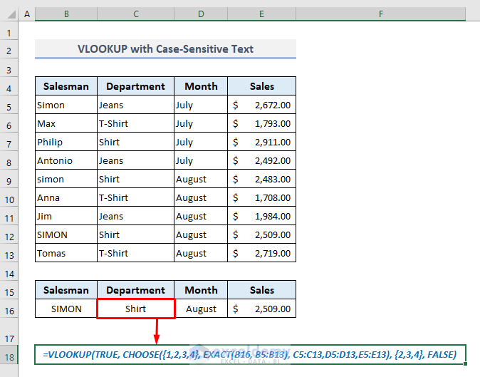
Example 1 – VLOOKUP to Find Case-Sensitive Text in Excel
We’ll look for the exact name ‘SIMON’ and draw out the sales data based on the match.
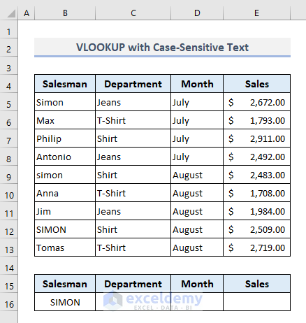
- The required formula in the output Cell C16 will be:
=VLOOKUP(TRUE, CHOOSE({1,2,3,4}, EXACT(B16, B5:B13), C5:C13,D5:D13,E5:E13), {2,3,4}, FALSE)- After pressing Enter you’ll be displayed the corresponding sales data for the exact name ‘SIMON’ only.
How Does the Formula Work?
- The lookup array of the VLOOKUP function has been defined with the combination of CHOOSE and EXACT functions.
- The EXACT function here looks for the case-sensitive matches of the name SIMON in the range of cells B5:B13 and returns an array of:
{FALSE;FALSE;FALSE;FALSE;FALSE;FALSE;FALSE;TRUE;FALSE}
- CHOOSE function here extracts the entire table data but only the first column shows the boolean values (TRUE and FALSE) instead of the salesman names.
- VLOOKUP function looks for the specified boolean value TRUE in that extracted data and subsequently returns the available sales records based on the row number of the matched lookup value TRUE.
Example 2 – Use a Drop-Down List as VLOOKUP Values
Under the primary table, we’ll create two drop-downs for the salesmen and months.
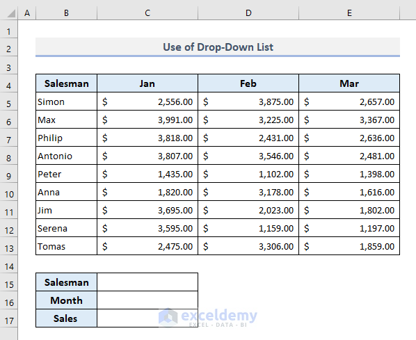
Steps:
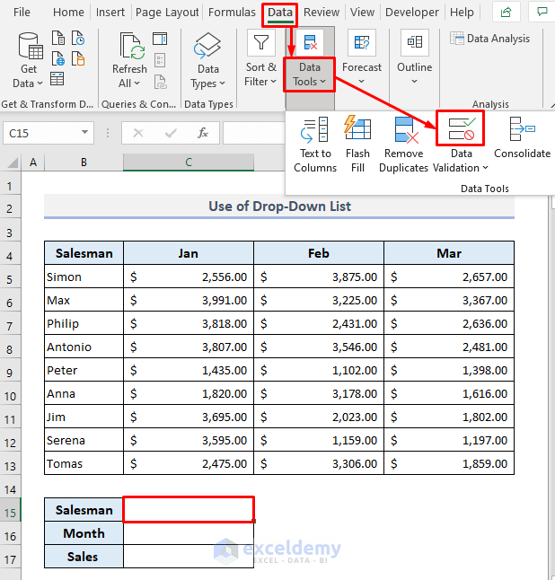
- Select Cell C15 where the drop-down list will be assigned.
- From the Data ribbon, choose Data Validation from the Data Tools drop-down.
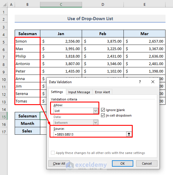
- A dialog box will appear.
- In the Allow box, select the option List.
- In the Source box, specify the range of cells containing the names of all salesmen.
- Press OK.
- You’ll find a drop-down list for all salesmen.
- Create another drop-down list for the range of cells (C4:E4) containing the names of the months.
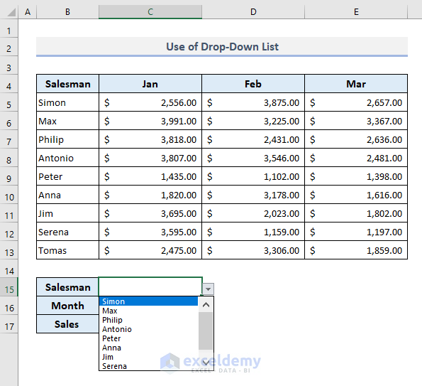
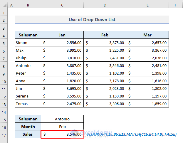
- Select the name Antonio from the Salesman drop-down.
- Select the month name Feb from the Month drop-down.
- In the output Cell C17, the corresponding formula will be:
=VLOOKUP(C15,B5:E13,MATCH(C16,B4:E4,0),FALSE)- Press Enter.
Things to Keep in Mind
- The lookup_value can be a single value or an array of values. If you enter an array of values, the function will look for each of the values in the leftmost column and return the same row’s values from the specified column.
- The function will look for an approximate match if the [range_lookup] argument is set to 1. In that case, it will always look for the lower nearest value of the lookup_value, not the upper nearest one.
- If the col_index_number is a fraction in place of an integer, Excel itself will convert it into the lower integer. But it will raise #VALUE! error if the col_index_number is zero or negative.
Download the Practice Workbook
Related Articles
- VLOOKUP Example Between Two Sheets in Excel
- Transfer Data from One Excel Worksheet to Another Automatically with VLOOKUP
- VLOOKUP from Another Sheet in Excel
- How to Use VLOOKUP Formula in Excel with Multiple Sheets
- How to Remove Vlookup Formula in Excel
- How to Apply VLOOKUP to Return Blank Instead of 0 or NA
- How to Hide VLOOKUP Source Data in Excel
- How to Copy VLOOKUP Formula in Excel
<< Go Back to Excel VLOOKUP Function | Excel Functions | Learn Excel
Get FREE Advanced Excel Exercises with Solutions!

Hi,
I did not get the department, month, and sales value in a horizontal array at once with the formula =VLOOKUP(B16;B5:E13;{2\3\4};FALSE) as {2\3\4} doesnt work. What version of Excel did you use when ve created this tutorial? Excel 2019 ?
Hi, Marian. All our Excel-related contents on this website have been made using Excel 365. I suggest you try the formulas in Excel 365 or Excel 2021 version. Thanks!