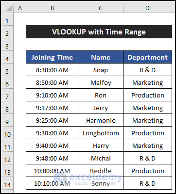
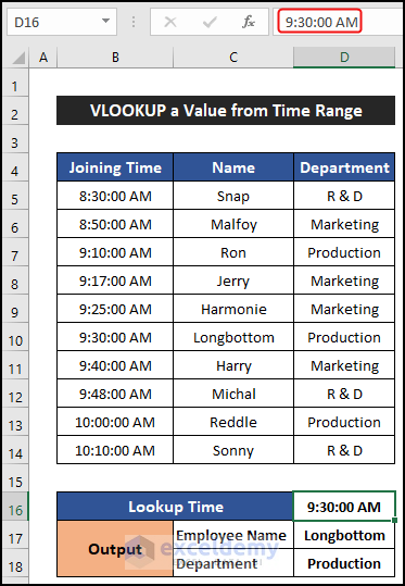
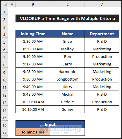
In this article, we will demonstrate five quick methods to VLOOKUP within a time range in Excel. To demonstrate the methods, we’ll use the dataset below of 10 employees of a company, including their Name, Department, and Joining Time on a particular day.
Note
All the operations in this article were performed using the Microsoft Office 365 application.
Method 1 – VLOOKUP a Value from a Time Range
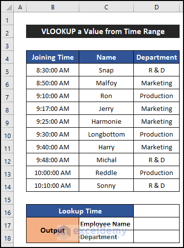
For the first example, we will input a Joining Time in cell D16, and the function will provide us with the name of the corresponding Employee and their Department in cells D17 and D18 respectively.
Steps:
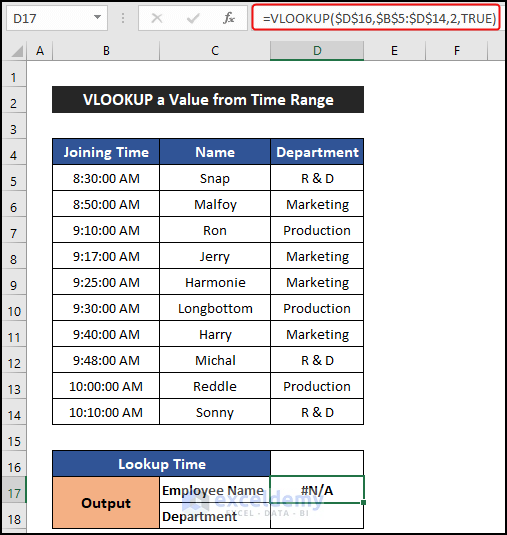
- In cell D17, enter the following formula:
=VLOOKUP($D$16,$B$5:$D$14,2,TRUE)
- Press Enter.
As we haven’t input a time yet, the function may show a #N/A error.
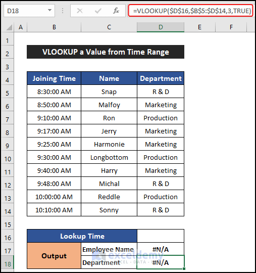
- In cell D18, enter the following formula to get the Department:
=VLOOKUP($D$16,$B$5:$D$14,2,TRUE)
- Press Enter.
- Enter a valid time in cell D16 and press Enter.
The Name and Department of the Employee whose Joining Time matches the input are displayed.
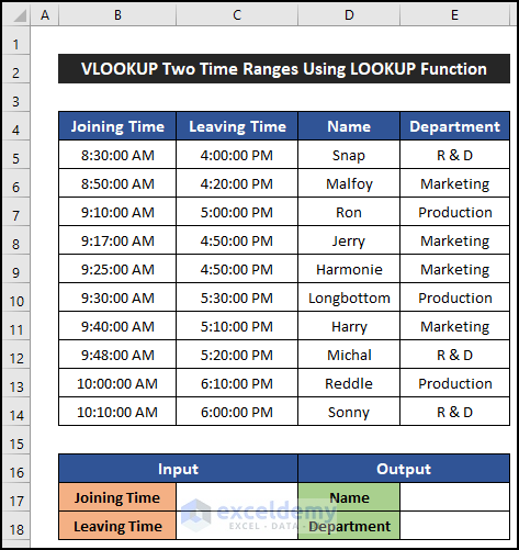
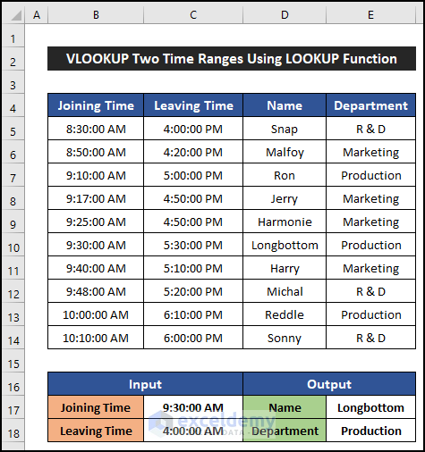
Method 2 – VLOOKUP from Two Time Ranges Using LOOKUP Function
Now we’ll use two different time ranges to VLOOKUP a value. For the second Time Range, we’ll add the Leaving Time of the employees to our dataset. We’ll input times in cells C17:C18 and return the output results in the range E17:E18.
Steps:
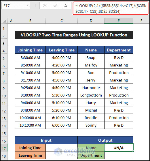
- In cell E17, enter the following formula:
=LOOKUP(2,1/($B$5:$B$14<=C17)/($C$5:$C$14>=C18),$D$5:$D$14)
- Press Enter.
As we haven’t input a time range in our input cells, the function may return an #N/A error.
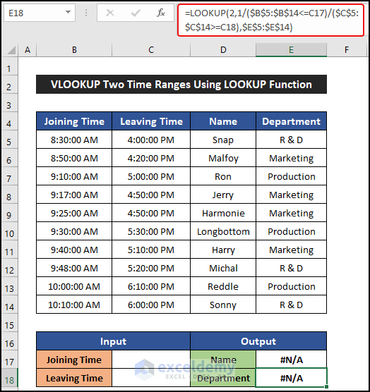
- In cell E18, enter the following to get the Department:
=LOOKUP(2,1/($B$5:$B$14<=C17)/($C$5:$C$14>=C18),$E$5:$E$14)
- Press Enter.
- Enter a valid time range in cells C17:C18.
- Press Enter.
The Employee Name and Department matching the input cells are returned in the output cells.
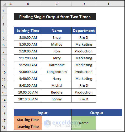
Method 3 – VLOOKUP a Single Output from Two Time Values
Now will use the INDEX, MATCH, and IF functions to return the value that lies between two input times. We’ll input the times in the range C17:C18 and get the output results in cells E17:E18.
Steps:
- In the merged cell E17, enter the following formula:
=INDEX(C5:C14,MATCH(1,IF(B5:B14>C17,IF(B5:B14<C18,1)),0))
- Press Enter.
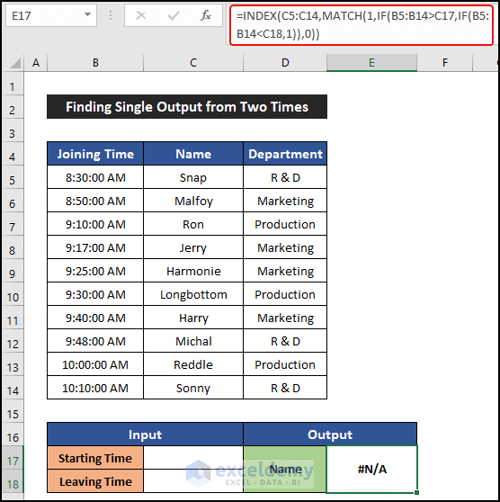
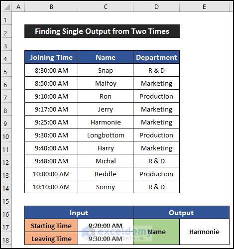
The name of the matching employee is returned.
Breakdown of the Formula
IF(B5:B14<C18,1): Checks whether the value of cell C18 is less than the time range. If true, the function returns 1. Otherwise, it returns FALSE. The formula returns 1.
IF(B5:B14>C17,IF(B5:B14<C18,1)): Checks whether the value of cell C17 is greater than the time range. If the logic is true, the function checks the second condition. Conversely, it returns FALSE. The formula returns 1.
MATCH(1,IF(B5:B14>C17,IF(B5:B14<C18,1)),0): Returns the row in which both conditions are met. The formula returns 5.
INDEX(C5:C14,MATCH(1,IF(B5:B14>C17,IF(B5:B14<C18,1)),0)): Shows the value of the cell in the row returned by the MATCH function. The formula returns Harmonie.
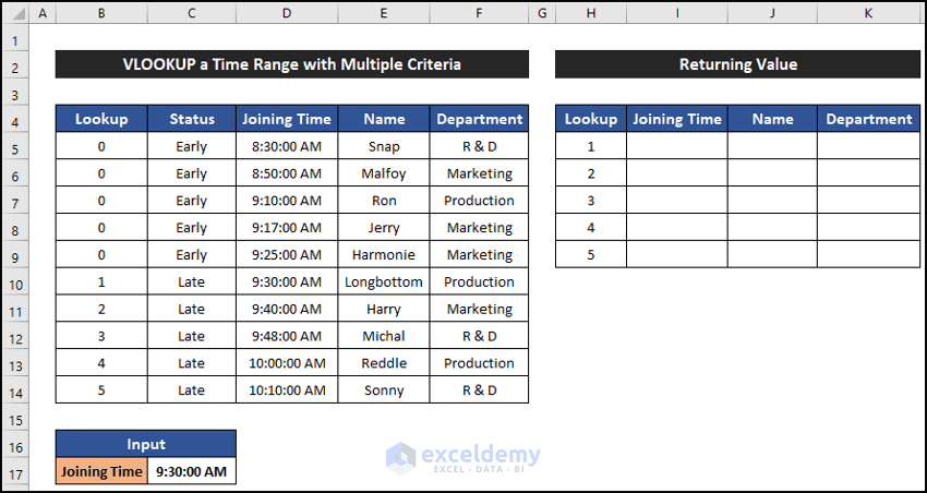
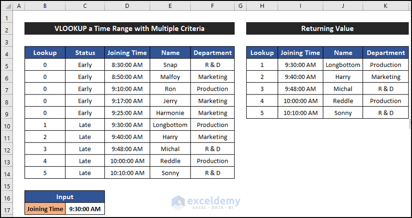
Method 4 – VLOOKUP a Time Range with Multiple Criteria
Now we will apply multiple criteria to do a VLOOKUP with a time range using the IF, COUNTIF, MATCH, and VLOOKUP functions.
Steps:
- Input a joining time, for example 9:30:00 AM.
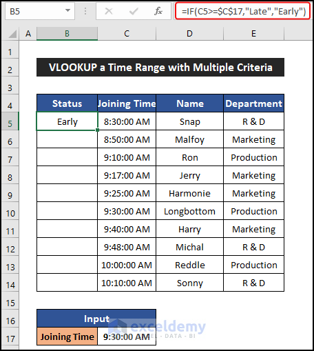
- Insert a column on the left side of our dataset titled Status.
- In cell B5, enter the following formula:
=IF(D5>=$C$17,"Late","Early")
- Press Enter.
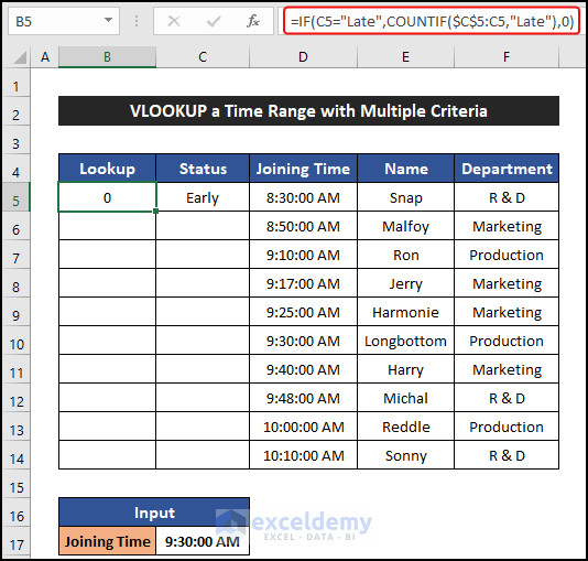
- Add another column on the left side of the dataset and title it Lookup.
- Enter the following formula in the first cell:
=IF(C5="Late",COUNTIF($C$5:C5,"Late"),0)
Breakdown of the Formula
COUNTIF($C$5:C5,”Late”): Counts the ‘Late’ values in column C. The formula returns 1.
IF(C5=”Late”,COUNTIF($C$5:C5,”Late”),0): Checks the value of the cell. If the cell value is ‘Late’ the COUNTIF function counts the value. Otherwise, it will show Zero (0). The formula returns 1.
- Press Enter.
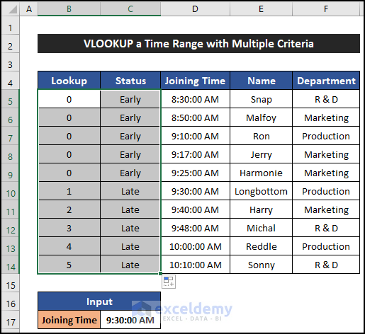
- Select the range of cells B5:C5 and double-click on the Fill Handle icon to copy the formula down to cell C14.
The first five values are Zero (0) and the last five values are numbered sequentially.
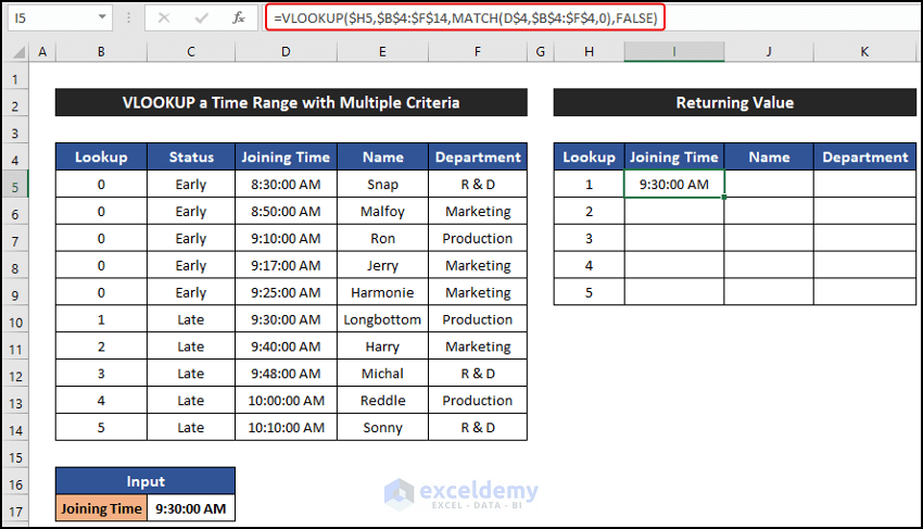
- Generate a new dataset like in the image below.
- In cell I5, enter the following formula:
=VLOOKUP($H5,$B$4:$F$14,MATCH(D$4,$B$4:$F$4,0),FALSE)
Breakdown of the Formula
MATCH(D$4,$B$4:$F$4,0): Searches for the exact match of the column heading in the main dataset and returns the column number. The formula returns 3.
VLOOKUP($H5,$B$4:$F$14,MATCH(D$4,$B$4:$F$4,0),FALSE): Uses the value provided by the MATCH function and extracts the corresponding value from the main dataset. The formula returns 9:30:00 AM.
- Press Enter.
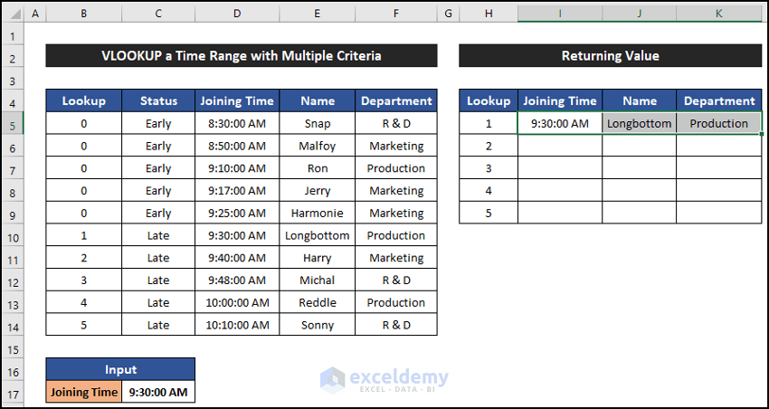
- Drag the Fill Handle icon to the right to copy the formula to cell K5.
- Select the range I5:K5 and drag the Fill Handle icon down to cell K9.
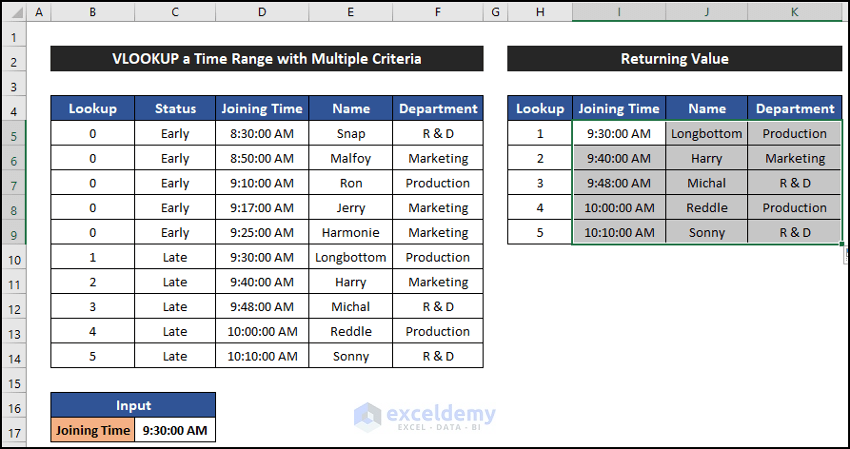
All the values are filled in the output location.
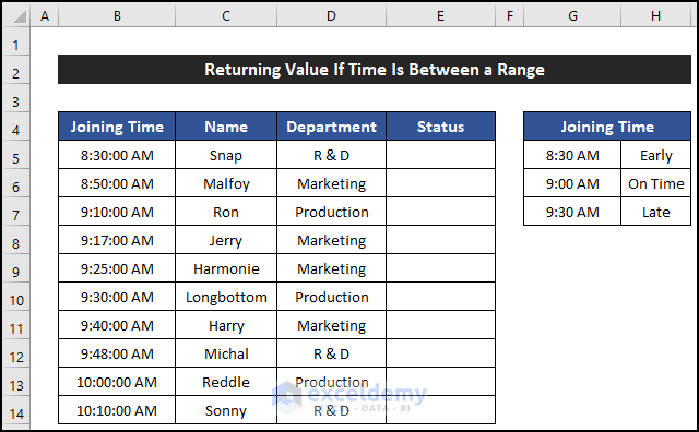
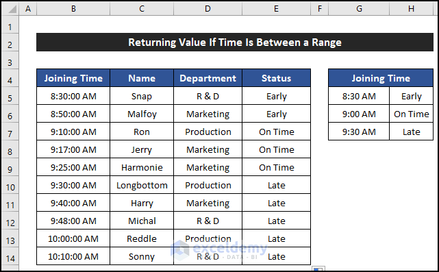
Method 5 – Return Value If Time Is Between a Range
In the final example, we will VLOOKUP data in a different dataset and extract a value into our dataset using the VLOOKUP function. Our main dataset is in the range of cells B5:D14 and the dataset from where we will import the values is in the range of cells G5:H7. We’ll display that data in column E.
Steps:
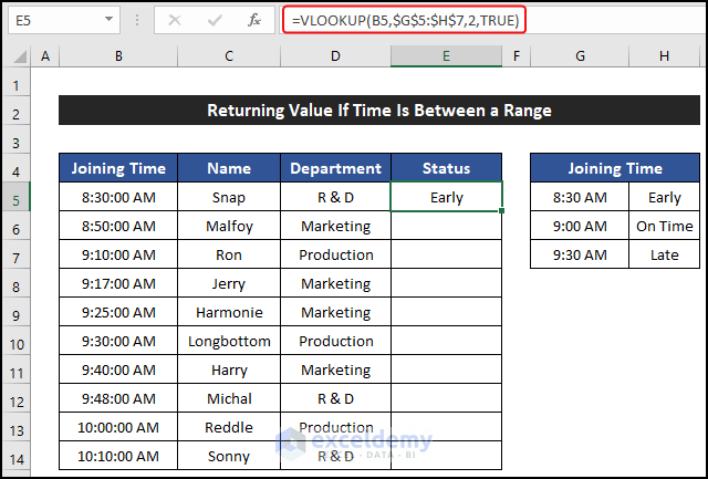
- In cell E5, enter the following formula:
=VLOOKUP(B5,$G$5:$H$7,2,TRUE)
- Press Enter.
- Double-click on the Fill Handle icon to copy the formula down to cell E14.
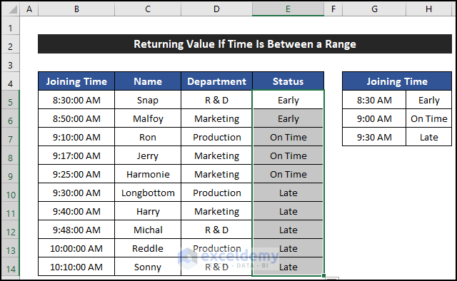
- All the values are extracted at the specifed location.
Download Practice Workbook
Related Articles
- How to Use VLOOKUP to Find a Value That Falls Between a Range
- How to Use VLOOKUP If Condition Lies Between Multiple Ranges in Excel
<< Go Back to VLOOKUP a Range | Excel VLOOKUP Function | Excel Functions | Learn Excel
Get FREE Advanced Excel Exercises with Solutions!
