Latest Posts From Zahid Shuvo
This is an overview. Download Practice Workbook Merge.xlsx Merge VBA.xlsm How to Merge Excel Sheets in One File 1. Consolidate Data ...
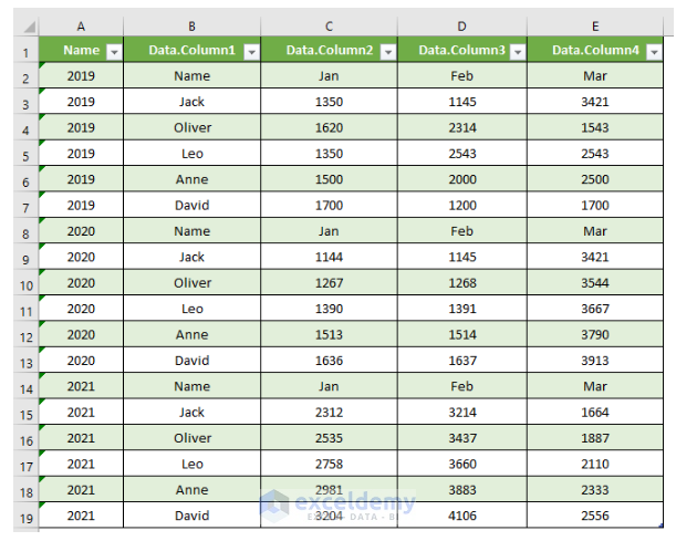
Method 1 – Using the Power Query Tool Below are two different tables for Physics A and Physics B. We will combine two tables from multiple worksheets with the ...

Excel Protected View feature acts as a barrier, protecting us from potential dangers when we open specific files. In this article, we'll look at how to ...

Method 1 - Change Display of Chart Axes 1.1. Display or Hide Axes Click the chart and select it. From the Chart Design tab, select Add Chart Element. ...

List of All Symbols in Excel This section lists all kinds of symbols, including those used in Excel formulas, characters, mathematical symbols, text and ...

Hi there! Are you tired of making Mailing Labels? Guess what you came to the right place. In this article, we will discuss all the steps of creating mailing ...
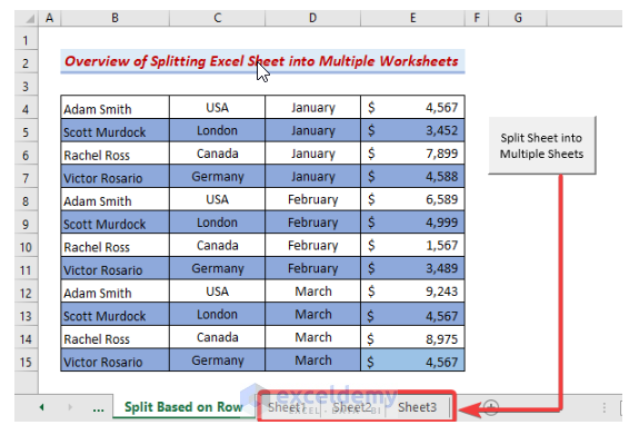
Here's an overview of splitting a large dataset so we can scroll independently across the panes. Download the Practice Workbook Split Sheet. xlsm ...

Finding matches is an integral part of data analysis. From searching out relevant information from a large dataset to finding errors by matching values, the ...

Mail Merge is a powerful feature in Microsoft Word that allows you to personalize and send the same document (such as emails or letters) to multiple ...
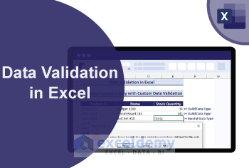
In this tutorial, you will learn everything about Data Validation from its purpose to how to apply it in your Excel worksheet. In the image above, we ...
This is an overview. 1. Using the “Save As” Command to Export Excel Data to Text or CSV File This is the sample dataset. To export ...

We'll use the following simple dataset to showcase how you can remove text. Download the Practice Workbook Text Remove.xlsx How to ...

In this Excel tutorial, you will learn how to: - Insert headers and footers - Use preset styles of headers and footers - Use custom styles for them - Edit ...

In the Pivot Table, a Slicer named Vendor was added. Its color was changed. What Is a Slicer in Excel A slicer is a graphical filtering ...
Method 1 - Custom Sort Slicer with Vendor Names Go to Options from File. Click on Advanced and click on Edit Custom Lists. Select cells ...
See Our Reviews at


Hi there, Nathalie!
Thanks for sharing your confusion here.
Since your problem seems unique. We have three possible cases of solutions that you can use.
Solution 01: You can use the Custom Sort feature to order the graph according to your choice. And it should update it by itself.
Solution 02: Add a new sunburst graph according to the sorted data if it does not work.
Solution 03: you can use sort data based on multiple columns, and you can specify secondary and tertiary sorting criteria. Here’s how:
Excel will first sort the data based on the primary column you specified. If there are any ties in the primary column, it will then sort those tied rows based on the criteria you specified for the secondary column, and so on for additional levels.
Then, add a new sunburst graph based on the newly sorted data.
Hopefully, one of the solutions from here should resolve your issue.
Regards
ExcelDemy Team
Hi CELIA!
To get your sheet to continue updating/moving over as you add more data to the original sheet, you must use a VBA Event. You can follow the steps to do it:
1. Press Alt + F11 to open the VBA editor.
2. Right-click on the Sheet1 module, choose “View Code,”
3. Paste the code into the code window.
In this code:
1. The Worksheet_Change event is triggered when changes occur in Sheet1.
2. The code checks if the change occurred in Sheet1 and if the changed range intersects with the specified range (e.g., columns A to Z).
3. If the conditions are met, it disables events to prevent infinite loops, clears Sheet2, and then copies the entire data from Sheet1 to Sheet2.
This way, when you delete items from Sheet1, Sheet2 will be updated to reflect the changes automatically.
Thanks for Reaching out to us.
Regards
Team ExcelDemy
Hey there!
We understand your problem that you shared here. Based on the scenario you have provided, there can be two possible cases of your problem and solution.
Case -1
If you want to convert the minute span into the tenths fraction of time as you mentioned. For example,
0-3 = .0
4-9 = .1
10-15 = .2
16-21 = .3
…….
58-60 = 1.0
You can simply use the formula to convert it into tenth fraction. (Yes, you are right, we will use multiple IF function to achieve it)
=IF(AND(A1>=0, A1<=3), 0, IF(AND(A1>=4, A1<=9), 0.1, IF(AND(A1>=10, A1<=15), 0.2, IF(AND(A1>=16, A1<=21), 0.3, IF(AND(A1>=22, A1<=27), 0.4, IF(AND(A1>=28, A1<=33), 0.5, IF(AND(A1>=34, A1<=39), 0.6, IF(AND(A1>=40, A1<=45), 0.7, IF(AND(A1>=46, A1<=51), 0.8, IF(AND(A1>=52, A1<=57), 0.9, IF(AND(A1>=58, A1<=60), 1, "Out of Range"))))))))))))
Replace A1 with the cell reference where your time value is located.
This formula uses nested IF statements to check the given conditions and return the corresponding result based on the specified ranges. If the value is outside the specified ranges, it will return “Out of Range.” Adjust the cell reference and the ranges as needed for your specific use case.
Case -2
In this case, if you want to convert the time 7:25:00 (hh:mm:ss) into 7.4. You can use the formula to convert it. Say, the value 7:25:00 is stored in cell A1.
=IF(AND(MINUTE(A1)>=0,MINUTE(A1)<=3),HOUR(A1)+0,IF(AND(MINUTE(A1)>=4,MINUTE(A1)<=9),HOUR(A1)+0.1,IF(AND(MINUTE(A1)>=10,MINUTE(A1)<=15),HOUR(A1)+0.2,IF(AND(MINUTE(A1)>=16,MINUTE(A1)<=21),HOUR(A1)+0.3,IF(AND(MINUTE(A1)>=22,MINUTE(A1)<=27),HOUR(A1)+0.4,IF(AND(MINUTE(A1)>=28,MINUTE(A1)<=33),HOUR(A1)+0.5,IF(AND(MINUTE(A1)>=34,MINUTE(A1)<=39),HOUR(A1)+0.6,IF(AND(MINUTE(A1)>=40,MINUTE(A1)<=45),HOUR(A1)+0.7,IF(AND(MINUTE(A1)>=46,MINUTE(A1)<=51),HOUR(A1)+0.8,IF(AND(MINUTE(A1)>=52,MINUTE(A1)<=57),HOUR(A1)+0.9,IF(AND(MINUTE(A1)>=58,MINUTE(A1)<=60),HOUR(A1)+1,"Out of Range")))))))))))
It will show 7.4 instead of 7:25:00.
You can use this formula for your dataset. To do so, replace A1 with the cell reference where your time value is located.
Thanks for choosing us. And we will be happy to solve your problem and answer your query regarding Excel.
Regards
ExcelDemy Team
Hey there, Mr. Connie!
Glad that you have shared you problem here.
You can keep the decimal places with the number by using the format below.
“#,##0.00”;“@” (Copy and Paste this)
But this will add double quotes at each cells of the dataset in Excel.
You have to use VBA macros to make the double quotes not visible in each cell when open in Excel but they’re there only when open in notepad.
Regards
ExcelDemy Team
Hey There, Mr. Mark.
Thanks for dropping your query here. You can follow the steps to copy the pivot table to the new book.
Regards
ExcelDemy Team
Hi there, Mr. Ronaldo!
Thanks for sharing your problem with us.
Excel’s Solver tool is designed for optimizing mathematical problems, not exhaustively finding all the possibilities sums. While Solver can search for combinations meeting a target, it might not guarantee all solutions, especially in complex cases. Solver’s algorithms might find suitable solutions, but they might not explore all combinations.
For finding all possible combinations leading to a fixed result, especially with many variables (like you have 100 items), Solver may not be the best option. Consider alternatives like custom Excel VBA macros or external programming languages like Python.
Regards
ExcelDemy Team
Hi there, Mr. Smith
Thanks for sharing your problem here. We have a solution for you on this issue. You can use the code below. This will basically highlight the cell (where the Manager has made any change) with yellow background and red font, and also a comment showing the date and time when the change is done.
Code:
Private Sub Worksheet_Change(ByVal Target As Range)
Dim WRng As Range
Dim rg As Range
Dim commentText As String
commentText = “Time of change: ” & Format(Now, “hh:mm:ss AM/PM”)
Set WRng = Intersect(Application.ActiveSheet.Range(“a1:ff983”), Target)
If Not WRng Is Nothing Then
Application.EnableEvents = False
For Each rg In WRng
If Not VBA.IsEmpty(rg.Value) Then
rg.AddComment commentText
rg.Interior.Color = RGB(255, 255, 0) ‘ Yellow background
rg.Font.Color = RGB(255, 0, 0) ‘ Red font color
End If
Next
Application.EnableEvents = True
End If
End Sub
You can follow the steps to run the code:
● Press ALT + F11 to access the VBA editor.
● In the Project Explorer, find and select the desired worksheet.
● Copy and paste the code above.
● Save the File.
● Go back to the Excel worksheet.
● Perform actions that trigger the event (e.g., change cell values).
If you still have any problem with this code. Please can you be more specific about your needs in this case thus we can provide you with a much more relevant solution?
Thanks again for your patience.
Regards
ExcelDemy Team
Hey there, Mr. Chhavi.
Thanks a lot for your feedback.
“Here’s how to understand what they mean:
1. Price Variance: This shows how much the change in prices affected the total revenue. If it’s positive, it means the price increase helped make more money. If it’s negative, the price decrease hurts the revenue.
2. Volume Variance: This tells us how much the change in the number of items sold affected the total revenue. If it’s positive, it means selling more items boosted the revenue. If it’s negative, selling fewer items lowered the revenue.
3. Mixed Variance: Mix variance, also known as sales mix variance, reveals how the proportion of different products or services sold affected the revenue change. If it’s positive, it means the sales mix of products contributed favorably to the revenue change. If it’s negative, the sales mix had a less favorable impact on revenue.
By doing this analysis, you can figure out what caused the revenue to change, whether it was because of price changes, selling more or fewer items, or both. It helps businesses understand how their sales are performing and make decisions on pricing and sales strategies accordingly.”
I hope you have your answer here. And sorry for the inconvenience. We would love to hear from you again.
Regards
ExcelDemy Team
Hey there, Carissa!
Thanks for sharing your problem here. To solve the issue, you just need a small modification in the VBA code.
Follow the steps in the 3rd method mentioned in the article and make a change into the VBA code as follows.
And then run the code. It would work the way you want.
Regards
ExcelDemy Team
Hey there, Thanks for sharing your problem here. Try the following excel worksheet in the article
https://www.exceldemy.com/mortgage-calculator-with-extra-payments-and-lump-sum-excel/
and try to solve the issue with this excel template. and make sure to follow the instructions mentioned in the article.
If you have any queries regarding excel, feel free to share. Also, you can post your Excel-related problems in the ExcelDemy Forum (https://exceldemy.com/forum/) with images or Excel workbooks.
Regards
Exceldemy Team