Method 1 – Using the Power Query Tool
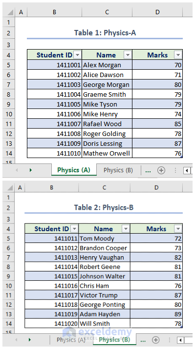
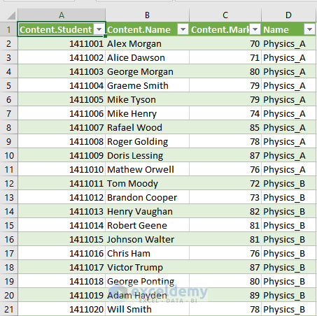
Below are two different tables for Physics A and Physics B. We will combine two tables from multiple worksheets with the Power Query Tool, combining the Physics marks from two sections of classes A and B.
Steps:
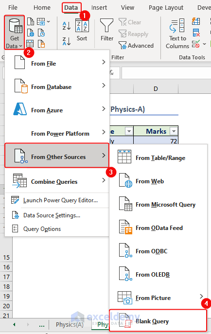
- From the Data tab, click on Get Data.
- From the drop-down menu, click on From Other Sources.
- Click on Blank Query.
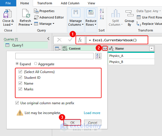
The Power Query Editor will appear as follows.
- Enter the following formula:
=Excel.CurrentWorkbook()- Click on the Double Arrow, as shown in the picture below.
- A dialogue box will appear. Check Select All Columns.
- Press OK.
- A combined dataset will appear in the Power Query Editor. Click on Close & Load.
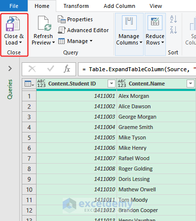
- A combined data table will appear in the new worksheet.
Method 2 – Using the VLOOKUP Function
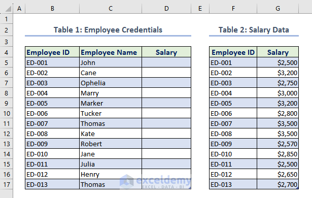
We have two tables: Table 1: Employee Credentials and Table 2: Salary Data in two separate worksheets. We will use the VLOOKUP function to combine these two tables into one common column.
Steps:
- Enter the following formula in cell E5:
=VLOOKUP($B5,'Lookup Table'!$B$5:$C$17,2,FALSE)- Press Ctrl+Shift+Enter.
How the Formula Works:
- $B2 is the value you are looking for.
- ‘Lookup Table’!$B$5:$C$17 is the table to search.
- 2 is the number of the column from which to extract the value.
- Rename the E column as Salary. The merged table will appear as follows.
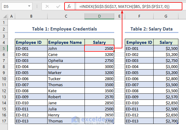
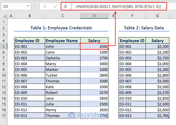
Method 3 – Using the INDEX MATCH Functions
Steps:
- Enter the following formula:
=INDEX($G$5:$G$17, MATCH($B5, $F$5:$F$17, 0))- Press Ctrl+Shift+Enter.
- The Salary column will merge with Table-1: Employee Credentials.
How the Formula Works:
Syntax: INDEX (return_range, MATCH (lookup_value, lookup_range, 0))
To modify the formula, change these parameters.
- Return_range : $G$5:$G$17
- Lookup_value : $B5
- Lookup_range : $F$5:$F$17
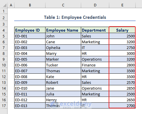
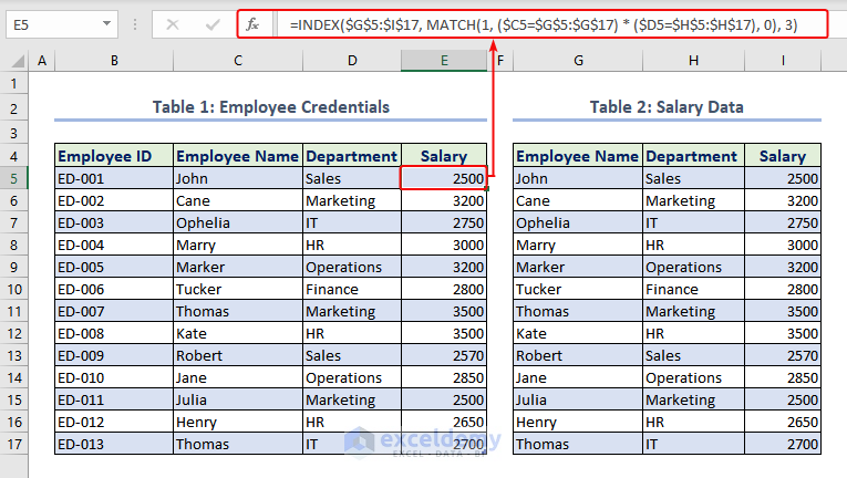
Method 4 – Matching Multiple Columns
Steps:
- Enter the following formula:
=INDEX($G$5:$I$17, MATCH(1, ($C5=$G$5:$G$17) * ($D5=$H$5:$H$17), 0), 3)- Press Ctrl+Shift+Enter.
- Salaries from Table 2 will be added to the Salary column of Table 1.
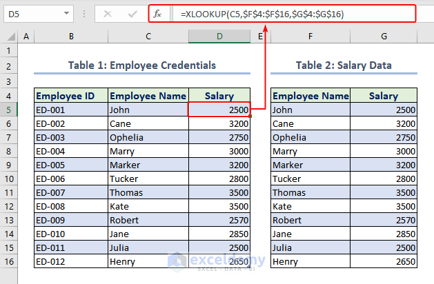
Method 5 – Utilizing the XLOOKUP Function
Steps:
- Enter the following formula in cell E5:
=XLOOKUP(C5,$F$4:$F$17,$G$4:$G$17)- Press Enter.
How the Formula Works:
- “C5” is the value you want to search for.
- “$F$4:$F$17″ represents the range of cells where you want to search for the value.
- “$G$4:$G$17” represents the range of cells from which you want to retrieve the corresponding value.
Things to Remember
- Check data accuracy and organization.
- Identify a common field/column.
- Sort both tables based on the common field/column.
- Back up your data.
- Choose the appropriate merge method (e.g., VLOOKUP, INDEX-MATCH).
Download the Practice Workbook
Merge Tables in Excel: Knowledge Hub
- Merge Two Tables in Excel and Remove Duplicates
- Merge Two Tables Based on One Column
- Merge Tables From Different Sheets
- Merge Two Tables in Excel Using Vlookup
- Merge Two Tables in Excel
<< Go Back to Merge in Excel | Learn Excel
Get FREE Advanced Excel Exercises with Solutions!

excellent work and satisfying.
Hello Samwel Gurt,
You are most welcome. We are glad to hear that our article is excellent and satisfying to you. You can explore more article related to these topic. Keep learning Excel with ExcelDemy.
Regards
ExcelDemy