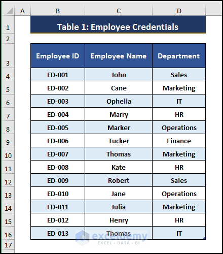
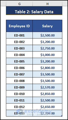
You have two separate Excel tables containing different data and want to merge these tables into one:
The VLOOKUP Function
The VLOOKUP function looks for values within an assigned range or table, organized vertically. It offers Approximate and Exact Matching for assigned values. The lookup values must be located in the first column. The syntax of the VLOOKUP function is
=VLOOKUP (lookup_value, table_array, column_index_num, [range_lookup])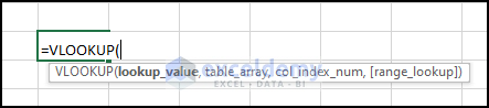
VLOOKUP Arguments
- lookup_value – the value you look for in the first column of an assigned range or table.
- table_array – the range or table from which you want to get the lookup_value.
- column_index_num – the column number within the range or table from which the value is returned.
- range_lookup – Approximate Match = TRUE (Default), Exact Match = FALSE [Optional]
Example 1 – Getting Data to Merge Two Equivalent Tables Using the VLOOKUP Function in Excel

Step 1
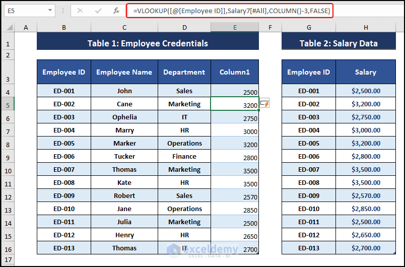
- Enter the following formula in any adjacent cell of the larger Table.
=VLOOKUP([@[Employee ID]],Salary7[#All],COLUMN()-3,FALSE)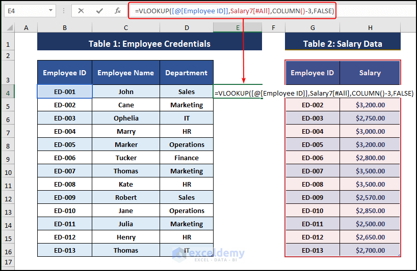
Step 2
- Press ENTER to display the output.
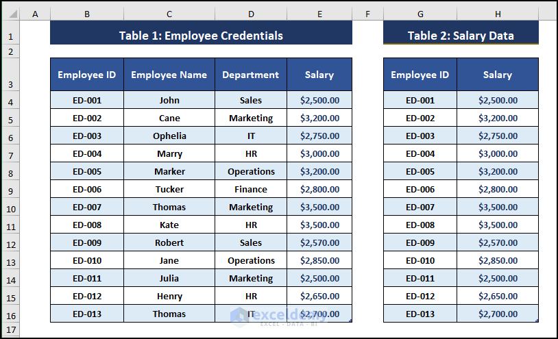
As data is formatted as a table, a column is added to the table.
This is the output.
Read More: How to Merge Two Tables in Excel
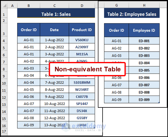
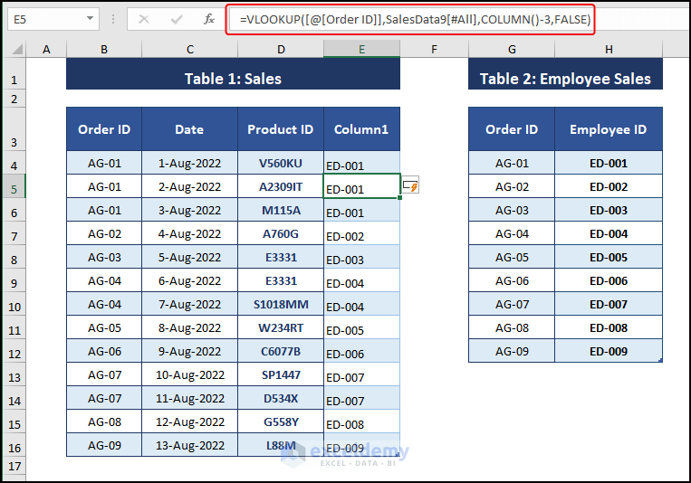
Example 2 – Merging Two Non-Equivalent Tables Using the VLOOKUP in Excel
Step 1
- Enter the following formula in any adjacent cell.
=VLOOKUP([@[Order ID]],SalesData9[#All],COLUMN()-3,FALSE)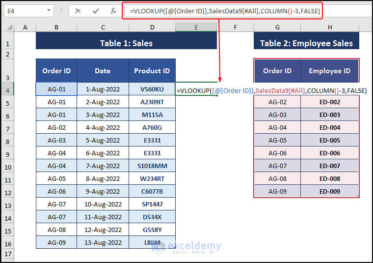
Step 2
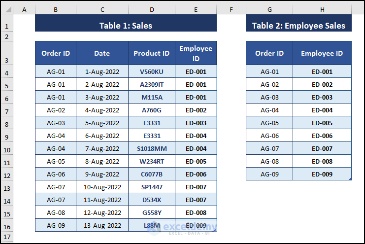
- Press ENTER to merge the table.
- Modify the table.
VLOOKUP Formula Explanation
=VLOOKUP([@[Employee ID]],Salary7[#All],COLUMN()-3,FALSE)
- [@[Employee ID]] = lookup_value.
- Salary7[#All] = table_array.
- COLUMN()-3 = column_index_num. The COLUMN function returns the column number of the cell in which the formula is entered (i.e., Column E = 5). 3 is deducted to get column data in the other table (5-3) or 2.
- FALSE = [range_lookup].
Read More: How to Merge Two Tables Based on One Column in Excel
Download Excel Workbook
<< Go Back to Merge Tables in Excel | Merge in Excel | Learn Excel
Get FREE Advanced Excel Exercises with Solutions!
