How to Merge, Find, and Unmerge in Excel: 9 Methods

Method 1 – How to Merge Cells in Excel Using Merge & Center Feature

• Select the cells from B5 to G5.
• Go to the Home tab. From the Alignment group, click the Merge & Center drop-down menu and click the Merge & Center command.

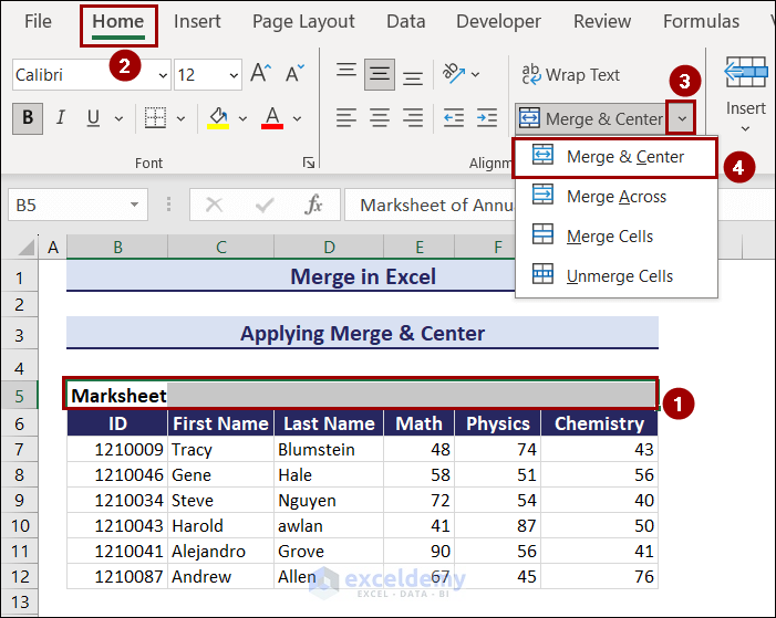
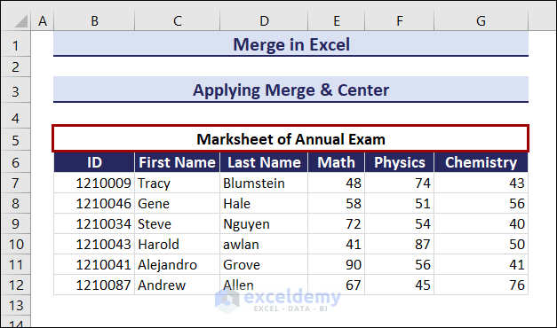
The selected cells will be merged into a single cell with the text centered, as seen in the picture below.

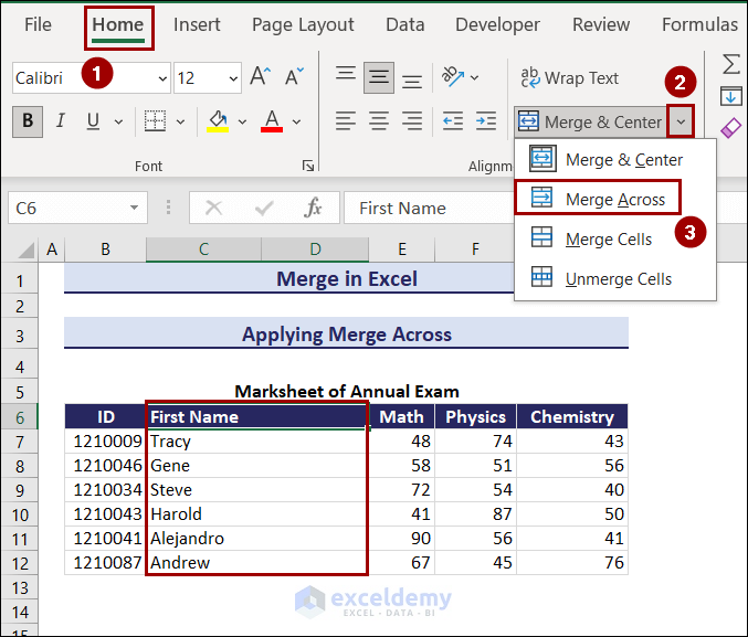
The Merge Across command merges cells only within each row of the selected range. If you select multiple rows and use the “Merge Across” command, each row’s cells will be merged independently.

Merge across the rows of the First Name and Last Name columns. Merge the cells of first and last names in each row and keep the first name only.

Click the Merge Across command from the Merge & Center dropdown.

• Get a warning from Microsoft Excel saying that “Merging cells will remove all the values except the upper-left value and discard other values.”
• If you believe that the other values are unimportant, click OK.
• Press the OK button repeatedly according to the size of the selected cells.

Apply the Merge Cells command to the selected cells like the previous two methods. The difference is that merging cells will merge the cells, keeping the upper left value only, and won’t center the data.

Method 2 – How to Merge Values from Multiple Columns in Excel

The previously mentioned method will potentially lose data while merging cells. If you combine the values of multiple columns while working with a large dataset. We will show you how to merge values from columns in Excel. No data will be lost while applying these methods.

– Using CONCAT Function
– Using the TEXTJOIN function

I. CONCAT Function

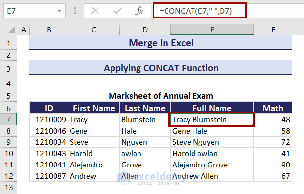
You have first and last names in this dataset in two columns. Combine the values from these two columns into a new column named Full Name. Use the CONCAT function to merge the values of two columns in Excel.

Steps:

• Select cell E7.
• Paste the following formula and press the Enter button.

• Drag the Fill Handle icon down to paste the used formula into the other cells of the column.

After applying the formula, you can see that the values of cells D7 and C7 are all present in cell E7.

II. TEXTJOIN Function

Use the TEXTJOIN function while combining the values of the columns.

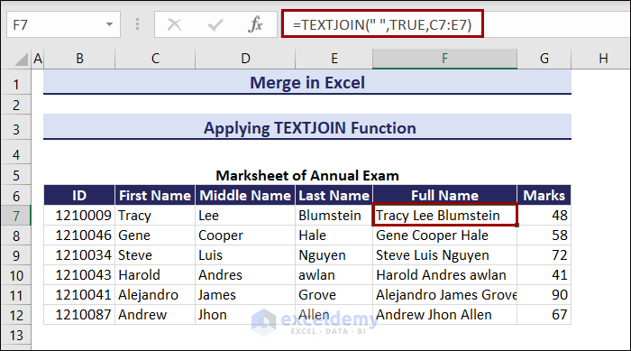
You have First Name, Middle Name, and Last Name in 3 different columns. Merge the values of these three columns and create the full name.

Steps:

• Select the F7 cell and write the formula below in the cell:

• Press the Enter button.

Observe that the data from the three cells is merged. Use the Fill Handle tool to apply the formula to the other cells.

Method 3 – How to Merge Rows by Using Justify Feature

You can also merge rows, like merging columns. Use Excel’s Justify feature to merge multiple rows without losing data.

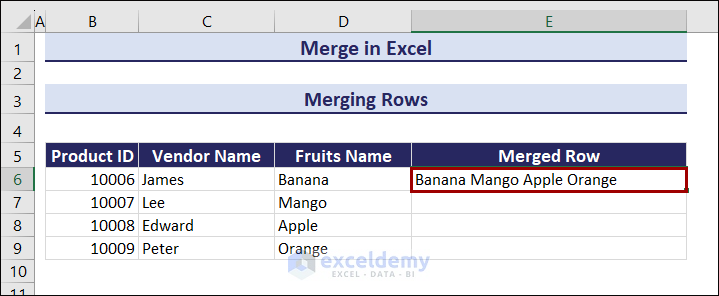
The rows of the D column contain some fruit names. Merge the data from these rows into a single cell now.

Follow the steps below.

• Select cells E6 to E9.
• Go to the Home tab >> from the Editing group >> click the drop-down of the Fill option >> select the Justify option.

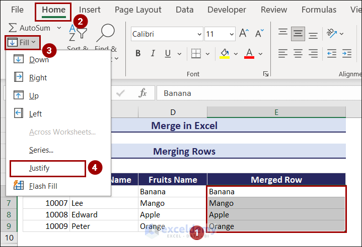
You can see the values of all the rows combined into a single row.

Method 4 – How to Merge Two Tables in Excel Using XLOOKUP Function

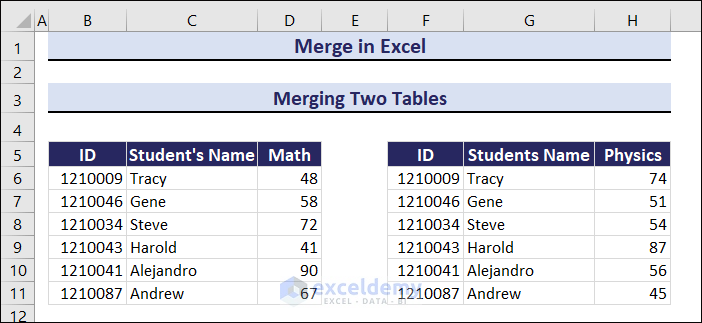
Merge data from multiple tables into one table. You’ll do this by using the XLOOKUP function. This method is applicable when both tables have similar fields.

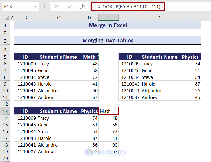
Two tables show the marks obtained by six students in their math and physics exams. These two tables will be combined to display the math and physics marks on the same table.

Follow the steps below to merge the tables:

• Copy any one table and paste it into your preferred place on the worksheet. Copy the second one that contains the physics marks. Add the math marks from the other table to this table.
• Select cell E13 and enter the following formula:

• Drag down the Fill handle to cell E19.

See that the two tables have been merged.

Method 5 – How to Merge Multiple Sheets in Excel Using VBA

Steps:

• Press Alt+F11 to open a new Microsoft Visual Basic for Applications window.
• Go to Insert and click on Module.

• A module window will appear. Now paste the following code:

Sub Merge_Multiple_Sheets()
Dim Worksheet() As String
ReDim Worksheet(Sheets.Count)
For i = 0 To Sheets.Count - 1
    Worksheet(i) = Sheets(i + 1).Name
Next i
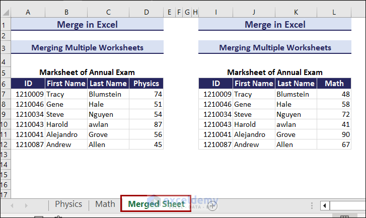
Sheets.Add.Name = "Merged Sheet"
Dim RowIndex As Integer
RowIndex = Worksheets(1).UsedRange.Cells(1, 1).Row
Dim ColumnIndex As Integer
ColumnIndex = 0
For i = 0 To Sheets.Count - 2
    Set Rng = Worksheets(Worksheet(i)).UsedRange
Rng.Copy
    Worksheets("Merged Sheet").Cells(RowIndex, ColumnIndex + 1).PasteSpecial Paste:=xlPasteAllUsingSourceTheme
    ColumnIndex = ColumnIndex + Rng.Columns.Count + 1
Next i
Application.CutCopyMode = False
End Sub
			

• Click the play button or press F5 to run the code.
• After running the code, you will see a new sheet named Merged Sheet has been created. The previous two sheets have been merged.

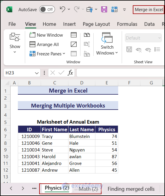
Method 6 – How to Merge Multiple Workbooks to One Workbook in Excel

Steps:

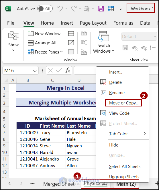
• Select the two sheets: Physics (2) and Math (2).
• Right-click on your mouse and select Move or Copy.

• A pop-up window named Move or Copy will appear.
• Go To book: drop-down box >> Select the workbook where you want to move or copy.
• Go to Before sheet: options >> Select the name of the sheet before which you want to paste the workbooks.
• Mark the Create a copy check box and press OK.

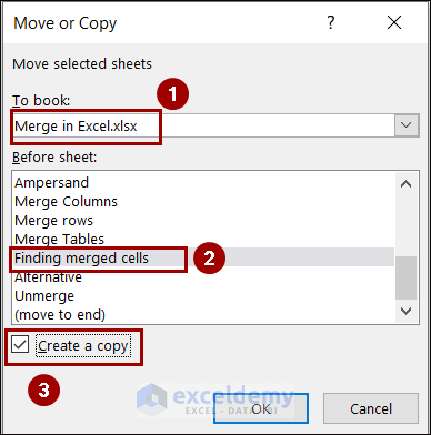
• The two sheets were copied to Merge in Excel‘s new workbook.

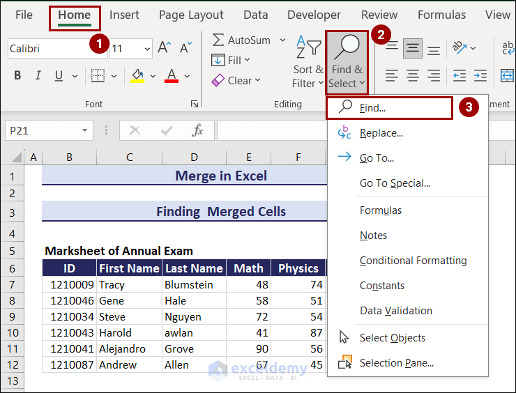
Method 7 – How to Find Merged Cells in Excel Using Find and Replace Feature

Steps:

• Go to the Home tab >> Editing group >> Select Find & Select drop-down >> click Find.

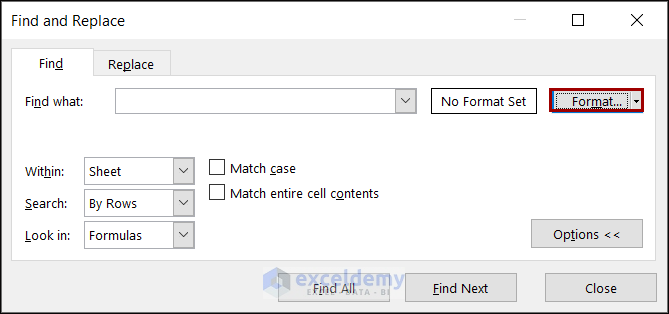
• A pop-up window named Find and Replace will appear.
• Select the Format drop-down box.

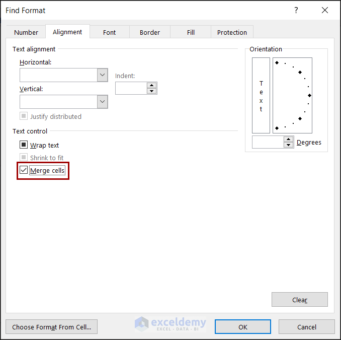
• The Alignment tab of the Find Format pop-up box will appear.
• Check the box for Merge cells under Text Control and press OK.

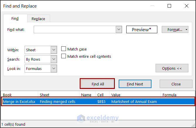
• Find and Replace will appear. Click Find All.
• See a list of all merged cells in your worksheet.

Method 8 – Alternative to Merge Cells in Excel: Center Across Selection

Steps:

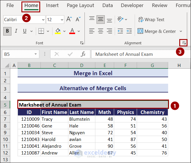
• Select the cells B5:G5.
• Go to the Home tab and click the Alignment Settings button.

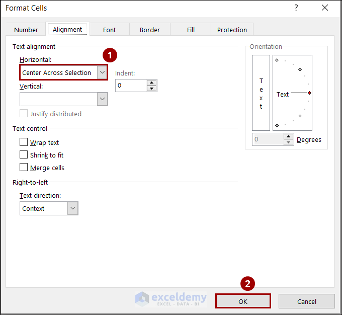
• The Format Cells window will appear.
• From the horizontal drop-down box, select Center Across Selection.
• Select the OK button.

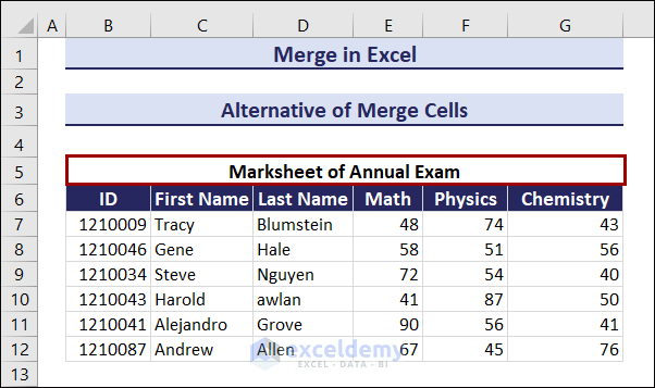
The selected cells have been merged.

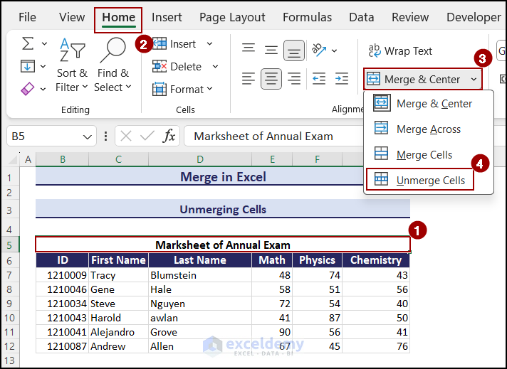
Method 9 – How to Unmerge Cells in Excel

• Select the merged cell B5.
• Go to the Home tab >> Click Merge & Center >> Select Unmerge Cells.

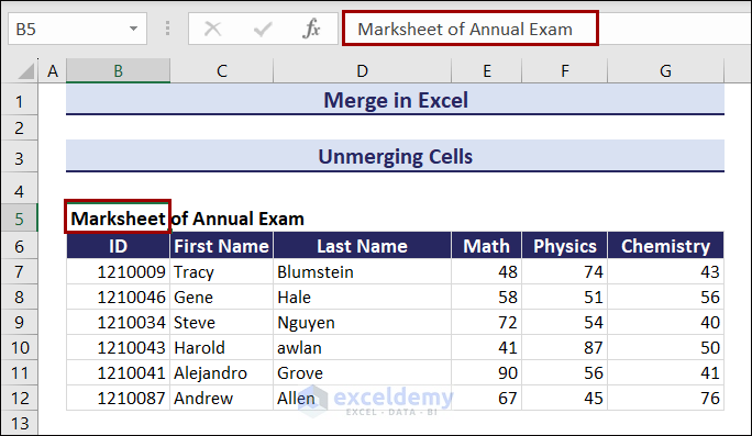
The merged cells are unmerged now.

Download Practice Workbook

Download the practice workbooks to exercise while you are reading this article.

Merge in Excel: Knowledge Hub

<< Go Back to Learn Excel