In this tutorial, I am going to show you 7 effective ways to merge two tables in Excel and remove duplicates. You can use these methods for small or relatively larger tables. They should work fine in all cases. Also, all of these methods take very little time to understand and apply as you will see in the following sections.
How to Merge Two Tables in Excel and Remove Duplicates: 7 Effective Ways
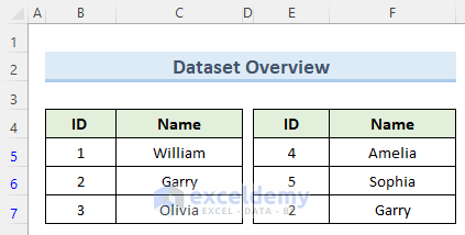
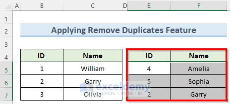
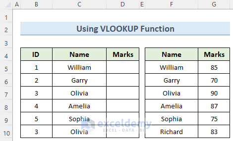
To explain the steps clearly and in a concise manner, we have taken a simple dataset in this tutorial. It has 4 rows and 5 columns which we will vary to some extent for the later methods. Also, make sure to format your dataset as a table which will make working with them a lot easier.
1. Use Advanced Filter Option
This option in Excel is the advanced version of the regular filter which helps to remove duplicates from tables. Let us see how to apply this option.
Steps:
- First, select the second table and press Ctrl+C to copy this table.
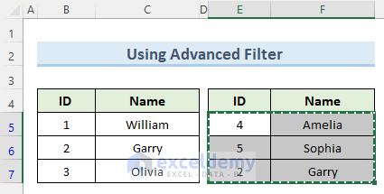
- Now, click on cell B8 and paste by using Ctrl+V.
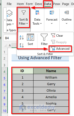
- Then, select the whole table go to the Data tab, and then Sort & Filter.
- Under this section, click on Advanced.
- Immediately, this will open the window, Advanced Filter.
- Here, select the Action to Filter the list, in-place.
- Next, insert the List range with your table range.
- Also, check the Unique records only and click OK.

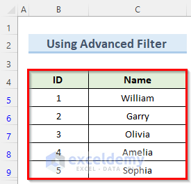
- Finally, this will remove all the duplicate records.
2. Applying Remove Duplicates Feature to Merge Two Tables in Excel
We can remove duplicates with a single click using the Remove Duplicates feature in excel. We will see in the below steps how to use this.
Steps:
- To start with, copy the second table as previously and paste it into cell B8.
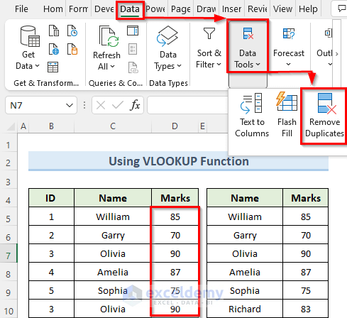
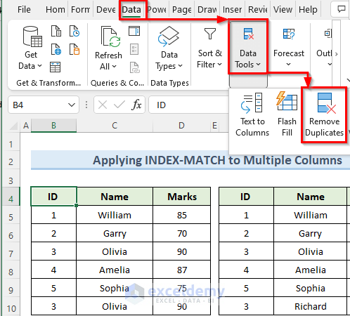
- Then, navigate to the Data tab and then Data Tools.
- Here, click on Remove Duplicates.

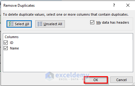
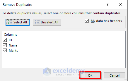
- Now, in the new Remove Duplicates window, make sure to check both columns’ titles and click OK.
- Consequently, this will remove all the duplicates and show a message. Press OK.

- Finally, you can check the table that there are no duplicates now.

Read More: How to Merge Two Tables Based on One Column in Excel
3. Utilizing Excel Power Query
If we want to merge two tables from different workbooks and then remove any duplicates, then the quickest way to do that is by using Power Query in excel. Here is how to use it.
Steps:
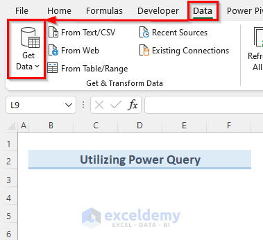
- First, navigate to the Data tab and then Get Data.
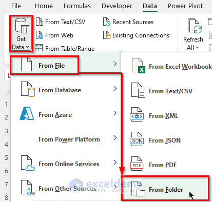
- Then, click on the drop-down and hover on From File.
- Here, select From Folder.
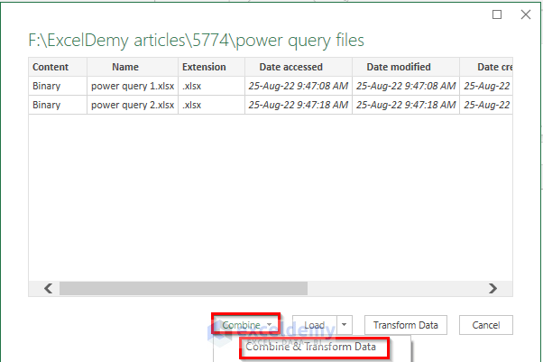
- Now, find the folder that contains the two workbooks with the tables and select Open.

- Next, you will see the two file name listed and click on Combine & Transform Data.
- Now, in the next window select a file from Sample File and click OK.
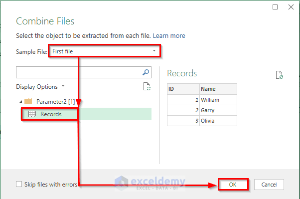
- Immediately, you will see the two tables have been merged in Power Query.

- Then, select the Name column and go to Remove Rows.
- Here, click on Remove Duplicates.
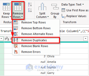
- As a result, Power Query will remove duplicate names.

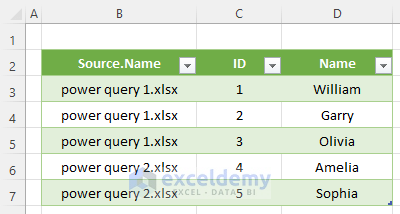
- Now, on the top-left corner click on Close & Load.

- Consequently, this will load the merged table in your excel worksheet.
4. Using VLOOKUP Function
The VLOOKUP function in excel can look up a specific value within a table that is organized vertically. We can use this to merge two tables and then remove the duplicates. Follow the steps below.
Steps:
- To begin with, go to cell D5 and type in the following formula:
=VLOOKUP(C5,$F$5:$G$10,2,FALSE)
- As a result, you should see that the data for the Name William is calculated.
- Then, drag the Fill Handle to copy the formula to the cells below.
- Next, from the Data tab, go to Data Tools and select Remove Duplicates as we saw previously.
- Then, confirm that all the columns are checked and click OK.
- Finally, excel will remove all the duplicates and give a confirmation message.

Read More: How to Merge Two Tables in Excel Using VLOOKUP
5. Combine INDEX and MATCH Functions
The INDEX function and the MATCH function in excel allow for performing advanced lookups which can help to merge two tables that have larger datasets.
Steps:
- First, double-click on cell D5 and enter the below formula:
=INDEX($G$5:$G$10, MATCH(C5,$F$5:$F$10,0))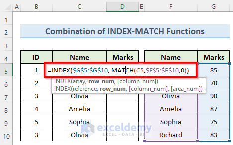
- Then, press the Enter key and copy the formula to the other cells below to bring all the data.
- Now, under the Data tab, go to Data Tools and then Remove Duplicates.
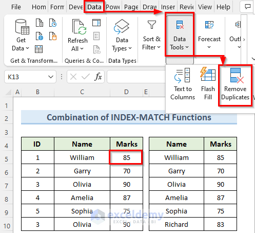
- Consequently, this will remove all the duplicates and show a confirmation window.

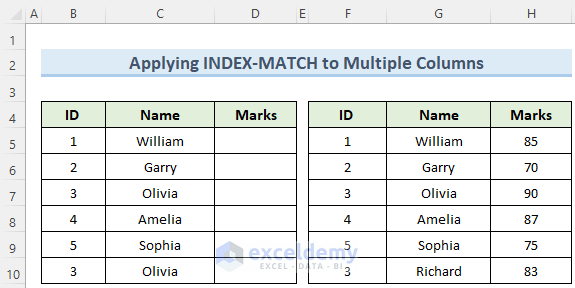
6. Merging Tables by Matching Multiple Columns
If we have two tables that have multiple columns in common, then we can use this method to merge them. Let us see how to do this.
Steps:
- To begin with, navigate to cell D5 and type in the below formula:
=INDEX($F$5:$H$10, MATCH(1,(B5=$F$5:$F$10)*(C5=$G$5:$G$10),0),3)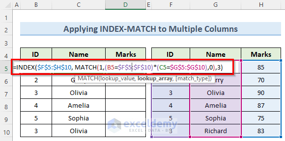
- Next, press Enter and copy the formula to the other cells below.
- Here, you can see the duplicate records in this table.
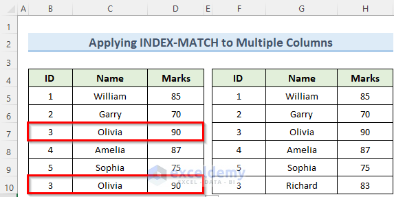
- As previously, select the whole table and click on Remove Duplicates under Data.
- As a result, you should no longer see any duplicate data.

7. Merge Tables and Remove Duplicates Using VBA Code in Excel
If you want to remove duplicates from multiple worksheets, then you can use VBA to achieve this very quickly. Let us see how we can write some VBA code for this.
Steps:
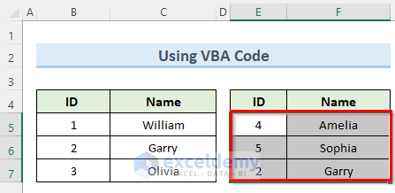
- First, select the second table and copy-paste it into cell B8.
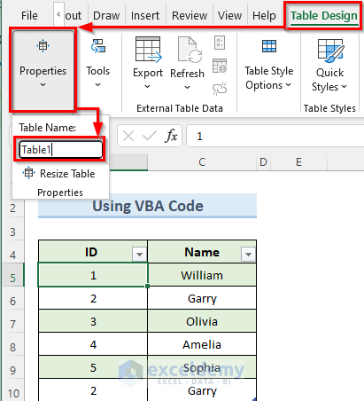
- Now, click anywhere on the table (it should be formatted as a table) and go to Table Design.
- Under the Properties section, set the Table Name as Table1.
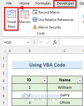
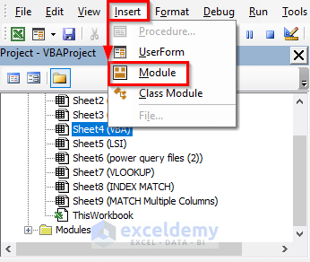
- Then, go to the Developer tab and click on Visual Basic.
- Then, in the VBA window, click on Insert and then Module.
- Now, in the new window, type in the following code:
Sub RemoveDuplicates_tables()
Dim ws As Worksheet
Dim tbl As ListObject
Set ws = ActiveSheet
Set tbl = ws.ListObjects(“Table1”)
tbl.Range.RemoveDuplicates Columns:=1, Header:=xlYes
End Sub
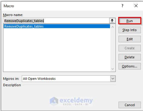
- Now, select Macros under the Developer tab.

- Then, in the new window, select the macro and click Run.
- Finally, you can see that the duplicates no longer exist.

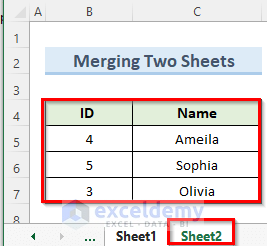
How to Merge Two Sheets into One in Excel and Remove Duplicates
In this method, we shall see how to bring data tables from different sheets and merge them into one sheet as a single table. Then we can use any of the previous methods to remove any duplicates.
Steps:
- To begin with, select and copy the table in Sheet2.
- Then, go to Sheet1 and paste the data under the Sheet1 table using Ctrl+V.
- Now, select the whole table in Sheet1 and click on Remove Duplicates under the tab Data.
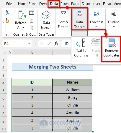
- Finally, this should remove the duplicates from the table.
Things to Remember
- Make sure to form your dataset as a table.
- If you have Excel 365, then you can use the XLOOKUP function instead of VLOOKUP.
- Remember to insert the $ sign otherwise, the formulas will not work.
Download Practice Workbook
You can download the practice workbook from here.
Conclusion
I hope that you understood the methods very well to merge two tables in Excel and remove duplicates. Try to apply these methods to larger datasets to save a lot of time. If you get stuck in any of the steps, I recommend going through them a few times. If you have any queries, please let me know in the comments.
<< Go Back to Merge Tables in Excel | Merge in Excel | Learn Excel
Get FREE Advanced Excel Exercises with Solutions!
