In this tutorial, you will learn everything about Data Validation from its purpose to how to apply it in your Excel worksheet.

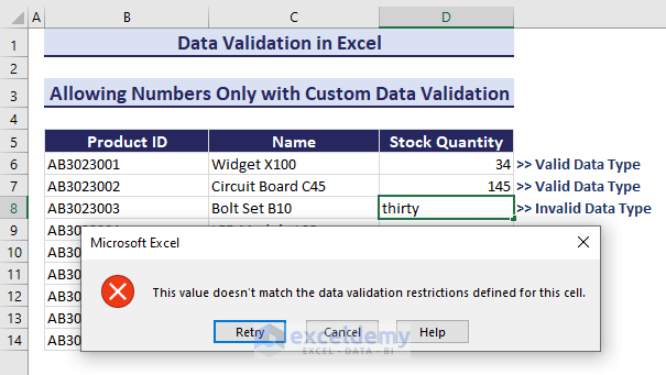
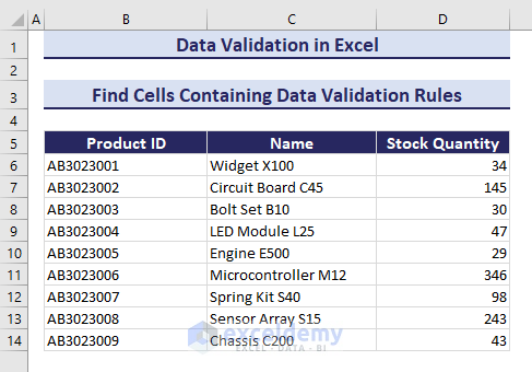
In the image above, we have applied the data validation in the column named “Stock Quantity” so it will store only numbers as input in the cells. If you enter any text value, it will show the message box saying, “This value doesn’t match the data validation restrictions defined for this cell”. That’s how data validation works.
⏷Data Validation in Excel
⏷Purposes for Using Data Validation
⏷Types of Data Validation Input
⏷1. How to Apply Data Validation in Excel?
⏵1.1. Apply Data Validation in Excel Cells
⏵1.2. Apply Multiple Data Validation Rules in One Cell
⏵1.3. Apply Data Validation Based on Another Cell
⏵1.4. Apply Data Validation with Checkbox
⏷2. Create a Drop-Down List with Data Validation
⏷3. Use Data Validation in Excel with Color
⏷4. Application of Custom Data Validation in Excel
⏵4.1. Allow Entries of Alphanumeric Characters Only with Data Validation
⏵4.2 Allow Numbers Only with Custom Data Validation
⏵Custom Excel Data Validation Rule Not Working
⏷5. Edit Data Validation
⏷6. Copy Data Validation to Other Excel Cells.
⏷Find Cells Containing Data Validation Rules
⏷Remove Data Validation in Excel?
⏷Useful Tips to Apply Data Validation
⏷Limitations of Data Validation
⏷Issues with Data Validation & How to Solve Them
Throughout this Excel blog post, you will learn how to
- Apply Data Validation (In cells, Multiple Rules, Rules based on another cell, With a Checkbox)
- Create a Drop-down list with Data Validation
- Use Data Validation
- Apply Custom Data Validation (Alphanumeric character only, Number Only)
- Edit Data Validation
- Find Data Validation
- Remove Data Validation
Note: We have used Microsoft 365 to prepare the dataset for this article. You can apply the mentioned methods in versions from Excel 2007 onwards.
What Is Data Validation in Excel?
Data validation in Excel is a feature that allows you to control the type of data entered into a cell. It helps maintain accuracy and consistency by setting rules for what can be input. For example, you can restrict entries to whole numbers, decimals, dates, or a predefined list.
What Is the Purpose for Using Data Validation in Excel?
We can use Data Validation in our Excel worksheet because it-
- stops us from entering incorrect data in cells.
- Keeps our data uniformly formatted.
- Simplifies and speeds up our data input.
- Enhances our overall data reliability.
- Creates a positive user experience.
- Allows custom rules using formulas for our unique requirements.
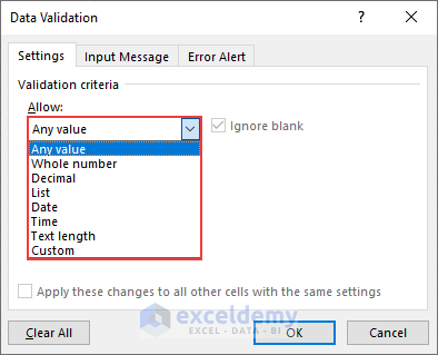
What Are All Types of Data Validation Input in Excel?
1 – The Settings Tab
There are two input boxes: Allow and Data. They set up the rules for data validation.
a) Allow Box:
You can choose the type of data validation:
- Whole Number: Allows only whole numbers.
- Decimal: Permits decimal numbers with a set precision.
- List: Creates a drop-down list that allows you to select from the list.
- Date: Ensures entries are within a specified date range.
- Time: Allows time only.
- Text Length: Controls the number of characters allowed.
- Custom: This lets you set unique rules using a formula.
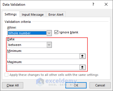
b) Data Box:
In the Data tab, you must define a criterion based on the validation you have selected in the Allow tab.
- Whole Number: Specify minimum and maximum values.
- Decimal: Set the number of allowed decimal places.
- List: Create a list of acceptable entries.
- Date/Time: Establish minimum and maximum date or time values.
- Text Length: Determine the minimum and maximum character count.
- Custom: Input a custom formula for validation.
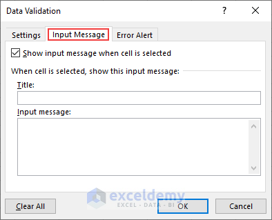
2 – The Input Message Tab:
You can use this tab to customize your message to give any instructions.
“Show input message when cell is selected” Box: Displays a message when users select the validated cell.
“Title and Input Message” Boxes: Customize the title and message of the notification.
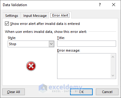
3 – The Error Alert Tab:
a) “Show error alert after invalid data is entered”: Ensures that the user gets a notification if they enter invalid information.
b) Style:
Choose the error alert type from this box:
- Stop (prevents entry)
- Warning (informs without blocking)
- Information (provides information without blocking).
c)Title and Error Message: Customize the title and message for the error alert.
Guide 1 – How to Apply Data Validation in Excel
- Select the cell or range where you want the validation.
- Go to the “Data” tab.
- Click on “Data Validation” and choose the validation type you need.
- Configure the criteria in all tabs based on your requirements and click “OK” to apply the validation.
Read on for more specific examples.
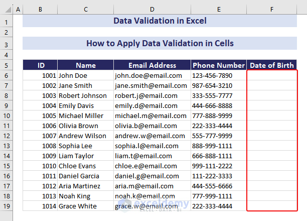
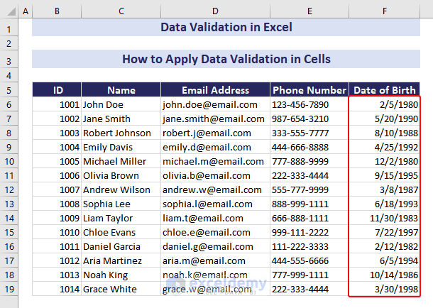
Case 1.1 – How to Apply Data Validation in Excel Cells
We have a dataset as below, where we’ll apply Data Validation in the column named “Date of Birth” to store dates only.
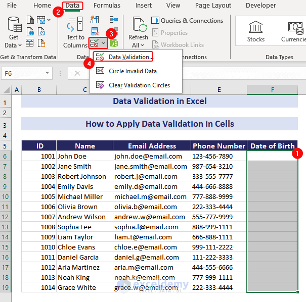
- Select the range F6:F19.
- Click on the Data tab and select Data Validation.
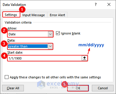
- Select Date in the Allow box.
- Select “greater than” in the Data box.
- Set 1/1/1900 (mm/dd/yyyy) as the Start date.
- Click on OK.
- The cells in the column will accept dates as inputs in the mm/dd/yyyy format. Otherwise, Excel will show an error message saying “This value doesn’t match the data validation restrictions defined for this cell.”
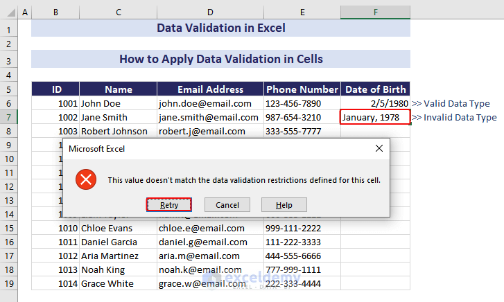
- If you enter proper data, it will allow it.
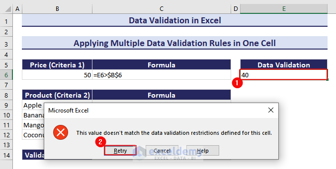
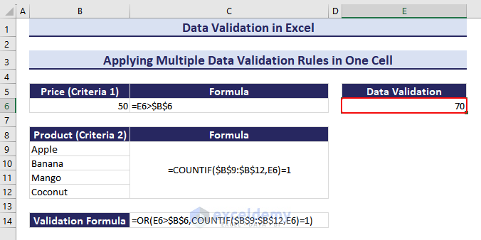
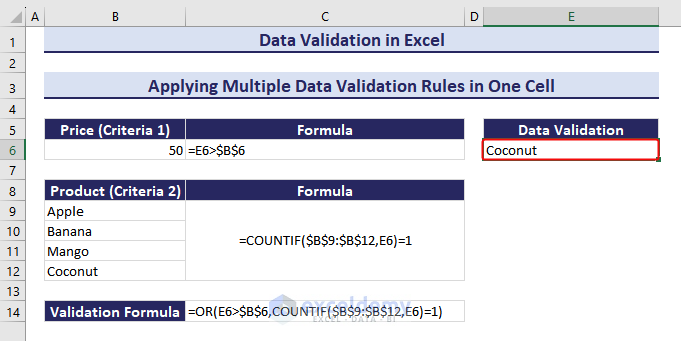
Case 1.2 – How to Apply Multiple Data Validation Rules in One Cell
We have a dataset below where we will take input and validate it in cell E6 based on Criteria 1 (Price greater than 50) and Criteria 2 (Product only from the list).
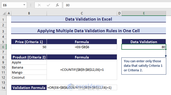
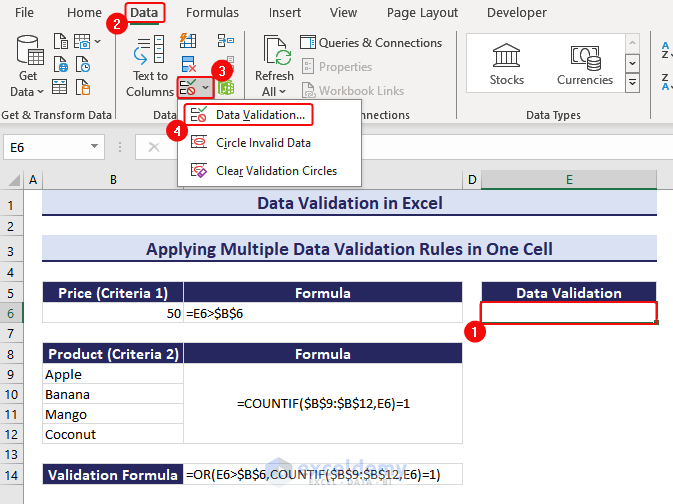
- Select cell E6.
- Click on the Data tab and go to Data Validation.
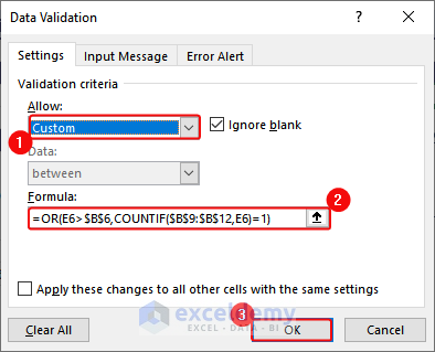
- Select Custom for Allow.
- Use the following formula in the Formula box:
=OR(E6>$B$6, COUNTIF($B$9:$B$12,E6)=1)- Click on OK.
- This will enable the Data Validation in cell E6. When you enter 40 in it, it will instantly show an error message, because it does not satisfy any of the criteria.
- When you enter 70 (which is greater than 50), it will accept this value as valid data since it satisfies Criteria 1.
- When you enter Coconut in cell E6, it will also accept it because it satisfies Criteria 2.
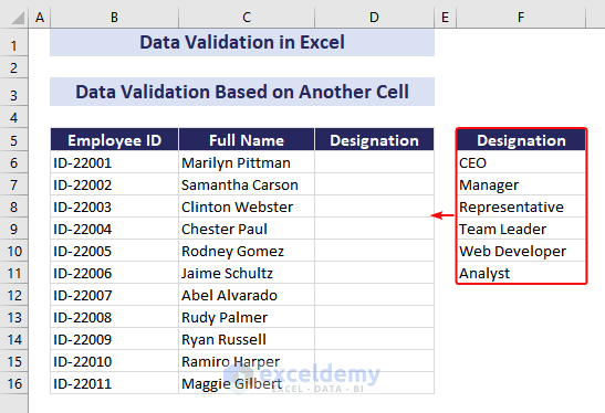
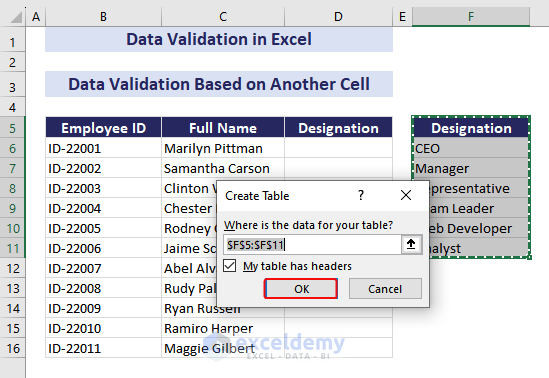
Case 1.3 – How to Apply Data Validation Based on Another Cell in Excel
Suppose we have data in cells F6:F11. We will use it to validate the values in the column named “Designation”.
- Select the range F5:F11.
- Press Ctrl + T.
- Check the My table has headers option.
- Click on OK.
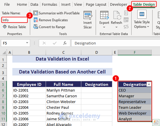
- Select the created table.
- Click on Table Design.
- Set the Table name as “Info”.
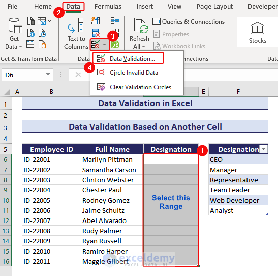
- Select the range D6:D16.
- Insert Data Validation.
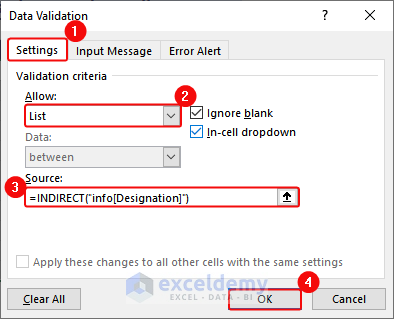
- Select List for Allow.
- Use the formula listed below in the Source box:
=INDIRECT(“Info [Designation]”)- Click on OK.
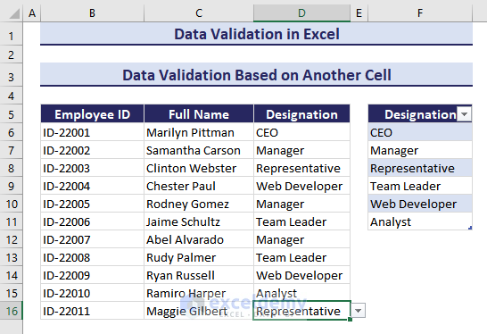
- This will create a drop-down list based on the table. Now in the column “Designation”, use the list to input the data.
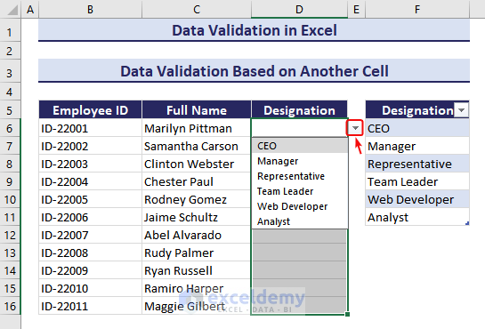
- You can choose values as you want.
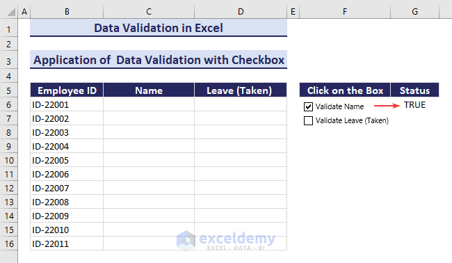
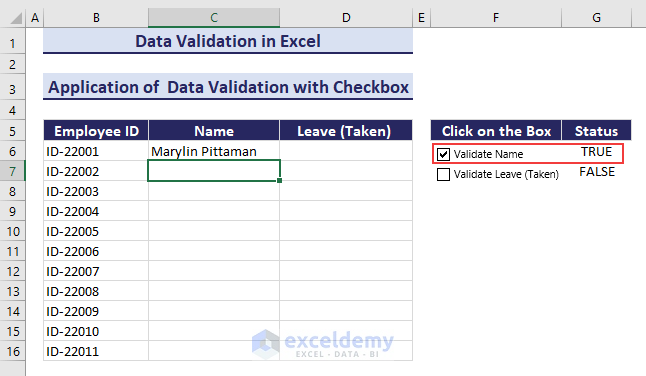
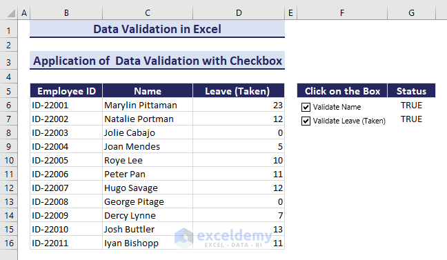
Case 1.4 – How to Apply Data Validation with a Checkbox in Excel
If you use a check box, you have to click on the check box to activate the data validation for the entry.
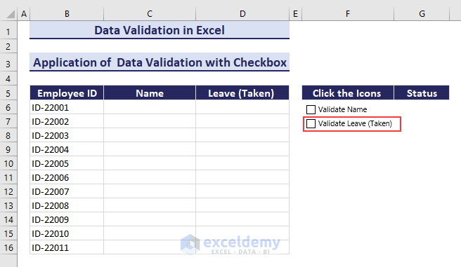
Consider the dataset below where we will apply Data Validation in the two columns named “Name” and “Leave (Taken)” using the check box.

- Go to Developer, Insert, and Check Box.
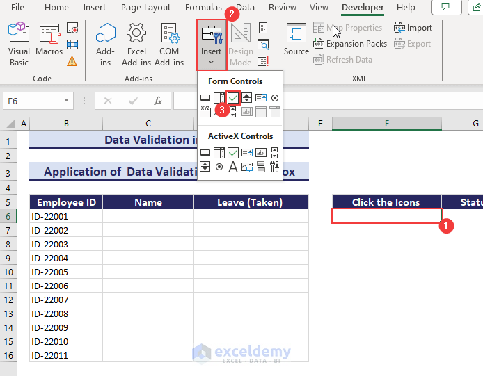
- Select the check box.
- Right-click and select Edit Text.
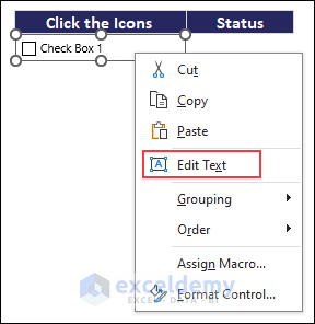
- Rename it as “Validate Name”.
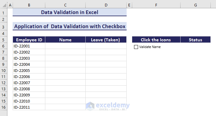
- Repeat to add another check box and rename it as “Validate leave (Taken)”.
- Select the first check box.
- Right-click and select Format Control.
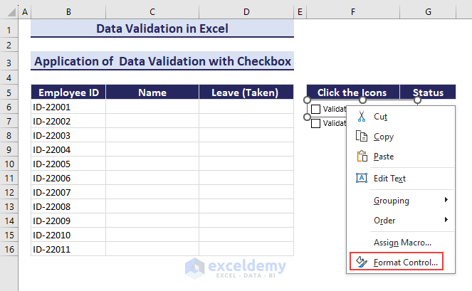
- Click on the Control tab in the Format Object dialogue box.
- Select cell $G$6 in the Cell link.
- Click on OK.
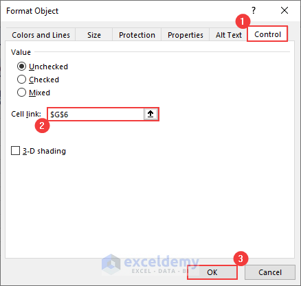
- Based on the check box, it will return TRUE or FALSE in the adjacent cell G6.
- Link G7 with the other check box named “Validate Leave (Taken)”.
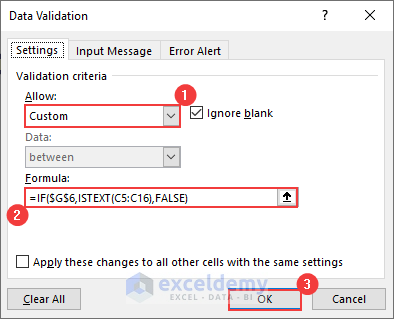
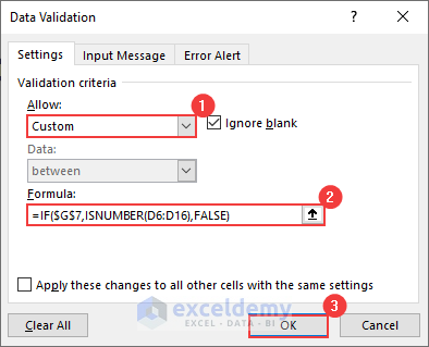
- Select the range C6:C16.
- Insert Data Validation.
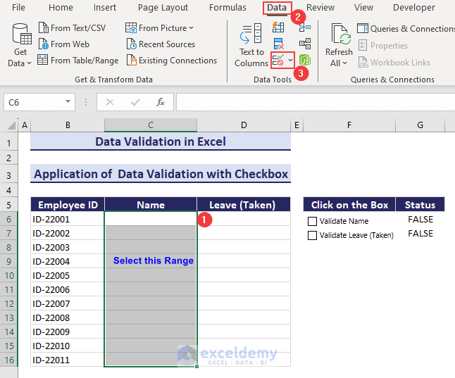
- Select Custom in the Allow box.
- Copy this formula in the Formula box:
=IF($G$6, ISTEXT(C5:C16),FALSE)- Click on OK.
- The Data Validation is activated. If you try to enter “Marylin Pittaman” in the “Name” column, it will return an error message box as we have not checked the “Validate Name” check box.
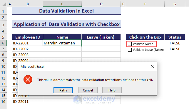
- When you check the “Validate Name” check box, it will take ‘Marylin Pittaman” as input. That’s how the check box validates the data entered in the cells of the “Name” column.
- Select the range D6:D16.
- Insert a new Data Validation.
- Select Custom in the Allow box.
- Copz the following formula in the Formula box.
=IF($G$7, ISNUMBER(D6:D16),FALSE)- Click on OK.
- When you uncheck the second check box, you cannot enter any number into the column “Leave (Taken)”.
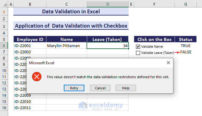
- If you check the “Validate Leave (Taken)” check box, it will allow you to enter any number into the cells.
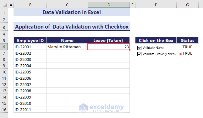
- By checking both checkboxes, you can enter the data in the columns. The result will be as the image below.
Guide 2 – How to Create a Drop-Down List with Data Validation in Excel
Suppose we want to make a drop-down list as shown in the figure below from existing data in the sheet.
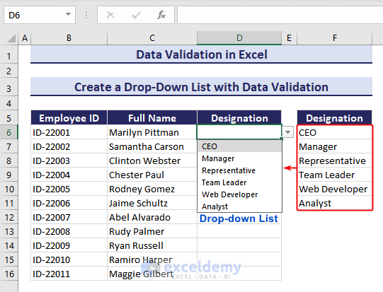
- Select the range D6:D16.
- Insert Data Validation.
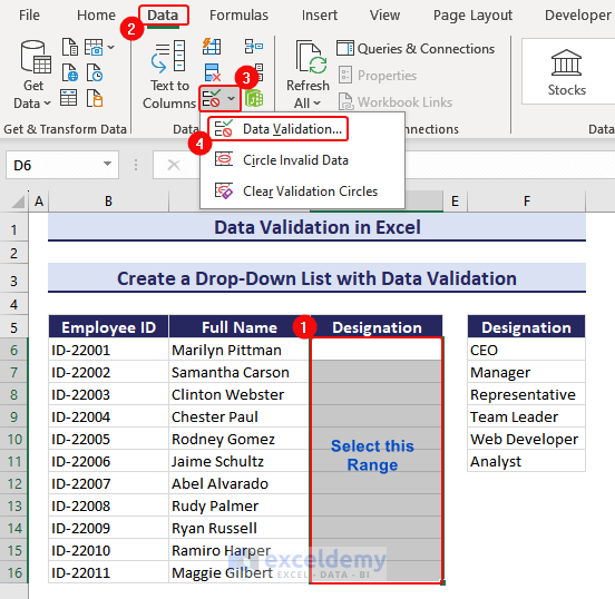
- Select List in the Allow box.
- Click on the Source icon.
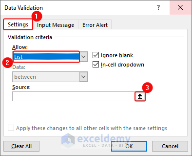
- Select the range F6:F11. These items will be added to the drop-down list.
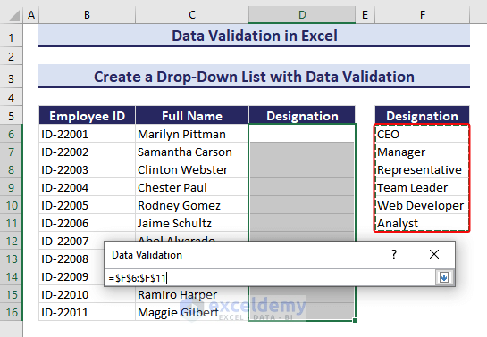
- Click on OK.
- Click on any cell.
- Select the drop-down icon on the right.
- A drop-down list will appear, and you can select your desired items.
![]()
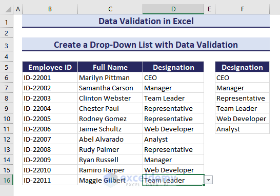
- We have used the drop-down list to fill up the column as shown in the image below.
Guide 3 – How to Use Data Validation in Excel with Color
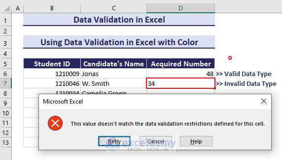
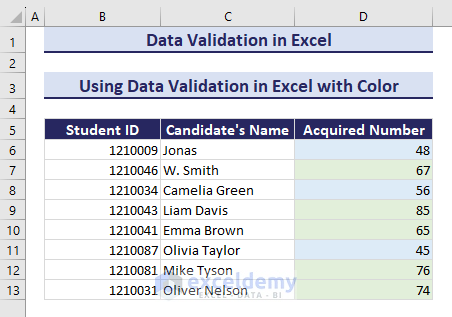
Suppose we have a dataset below. In the “Acquired Number” column, we will allow only the whole number (that is greater than 40) as input and highlight those values based on the condition using the Conditional Formatting.
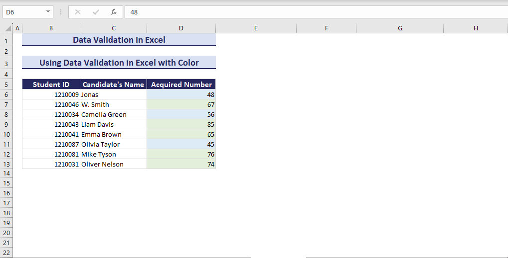
- Select the range D6:D16.
- Insert Data Validation.
- Select Whole number in the Allow box.
- Select between in the Data box.
- Set 40 as Minimum and 100 as Maximum.
- Click on OK.
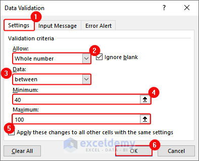
- This will enable Data Validation for this range. You can enter a number between 40 and 100. If you enter any number less than 40 (i.e.,34), it will return you an error message box.
- Select the range D6:D16.
- Click on Conditional Formatting and select New Rule.
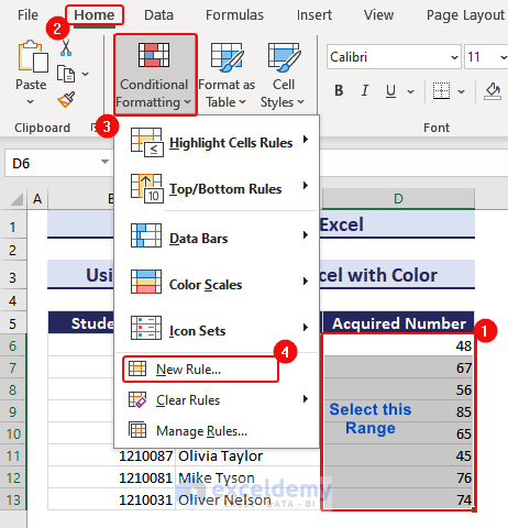
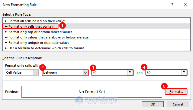
- Click on “Format only cells that contain”.
- Select between.
- Type the numbers 40 and 59 in the boxes under the “Format only cells within” option.
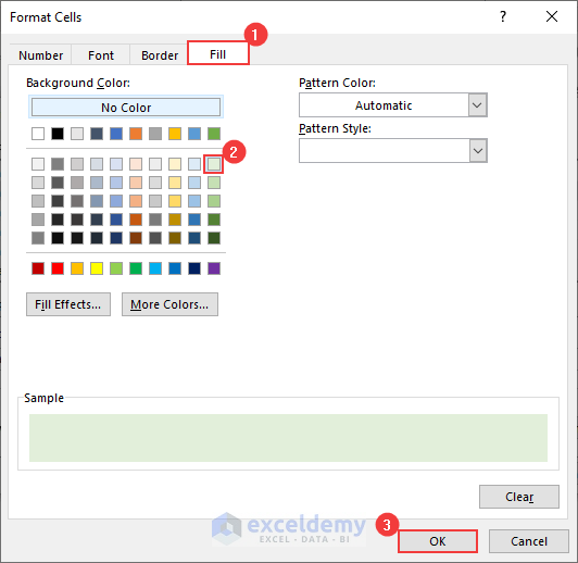
- Click on Format to add color.
- Click on Fill in the Format Cells dialogue box.
- Select the color you want.
- Click on OK.
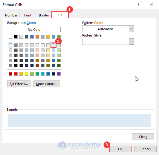
- Click on OK.
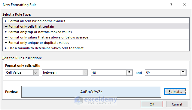
- In the column, it will highlight the numbers less than 60 with the selected color.
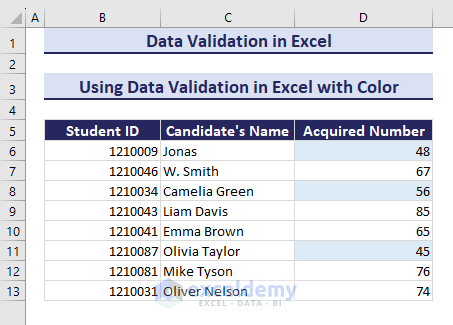
- Repeat for the range between 60 and 100 with a New Conditional Formatting Rule.
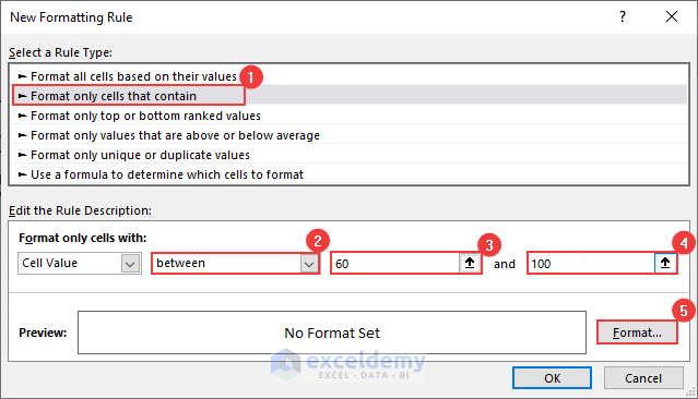
- Choose a different fill color.
- This will highlight the numbers greater than 60 with the selected color as shown in the image below.
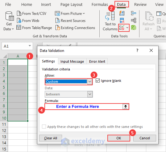
Guide 4 – Application of Custom Data Validation in Excel
We have set our rules/formula for the data from the Custom rules in the Data Validation dialogue box as shown in the image.
Case 4.1 – How to Allow Entries of Alphanumeric Characters Only with Data Validation
Alphanumeric characters are a combination of alphabetical (letters) and numerical (numbers) characters. We have a dataset below and will add Alphanumeric Characters in the “Model” column.
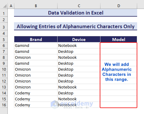
- Select the range D6:D16.
- Go to Data Validation.
- Select Custom in the Allow box.
- Use the following formula:
=ISNUMBER(SUMPRODUCT(SEARCH(MID(B5, ROW(INDIRECT("1:"&LEN(D6))),1),"0123456789abcdefghijklmnopqrstuvwxyzABCDEFGHIJKLMNOPQRSTUVWXYZ")))- Click on OK.
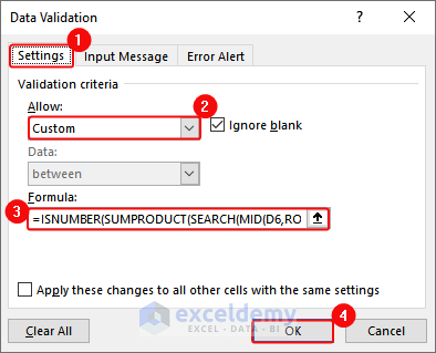
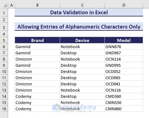
- This will allow only Alphanumeric characters in the range.
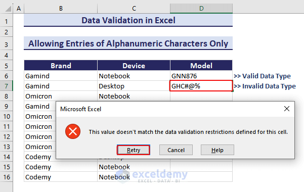
- We can only store the Alphanumeric characters in the cells.
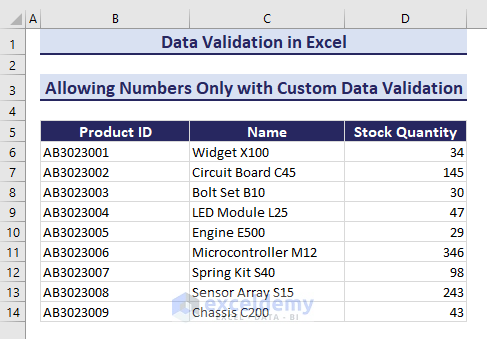
Case 4.2 – Allow Numbers Only with Custom Data Validation in Excel
Suppose we have a dataset as the image below. We want to allow only numbers in the column “Stock Quantity”.
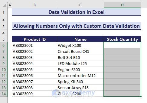
- Select the range D6:D14.
- Insert Data Validation.
- Select Custom in the Allow box.
- Use the following formula in the Formula box:
=ISNUMBER (D6:D14)- Click on OK.
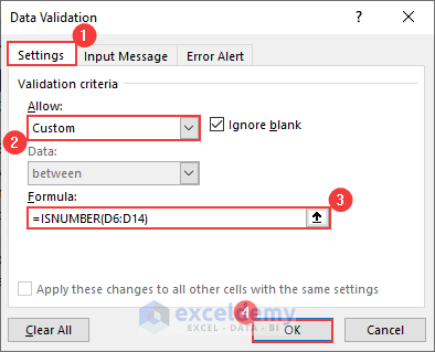
- This will allow only numbers into the cell of the column. Otherwise, it will show an error message.
- We have completed the dataset where the column “Stock Quantity” contains only numbers.
Custom Excel Data Validation Rule Not Working: Reasons & Solutions
- Ensure that the custom formula you entered is correct. Double-check for any syntax errors or typos in the formula.
- If your custom formula refers to other cells, make sure the cell references are accurate and that the referenced cells contain the expected values.
- Verify that you’ve selected the correct cell range for applying the data validation rule.
- Check if you’ve set up error alerts correctly in case the validation rule is violated. Sometimes, error alerts may not be visible, or the chosen alert style may not match the situation.
- Ensure that the cell format is appropriate for the validation rule. For example, if your rule checks for a date, the cell should be formatted as a date.
- If you are working with an older Excel version, be aware of compatibility mode issues. Certain features may not work as expected in compatibility mode.
- If the worksheet is protected, check if data validation changes are allowed. Sometimes, protection settings may restrict the application of new rules.
- Check for any conflicts with conditional formatting rules. Conflicting rules might override each other.
Guide 5 – How to Edit Data Validation in Excel
We have a dataset as below, with an existing drop-down list using Data Validation. We will edit it and add a new item “Representative” to the drop-down list.
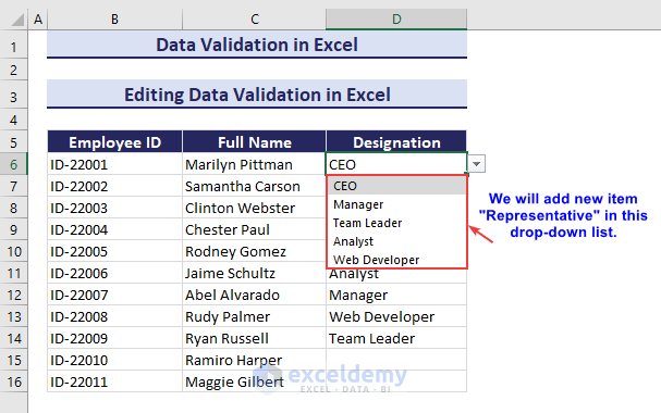
- Select any cell in the column “Designation”.
- Add “, Representative” in the Source box (including the comma).
- Check “Apply these changes to other cells with the same setting” to apply to the other cells.
- Click on OK.
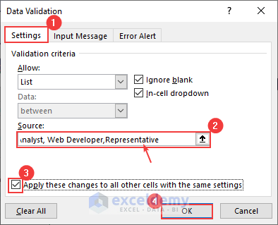
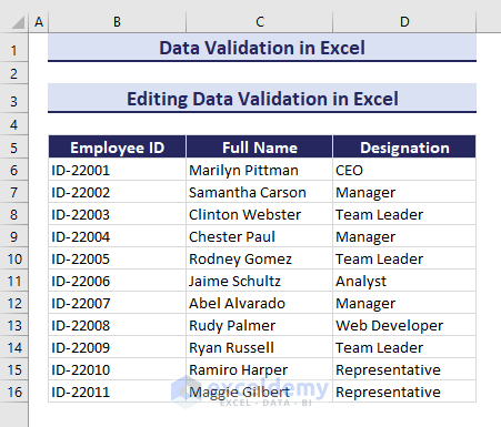
- This will add the new item “Representative” to the list.
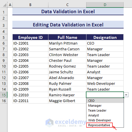
- You can use this list to complete data entry into the cell.
Guide 6 – How to Copy Data Validation to Other Excel Cells
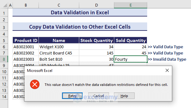
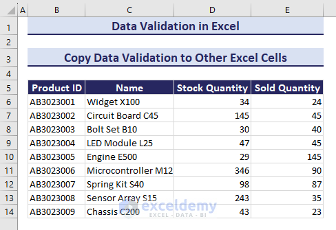
We have a dataset where the column “Stock Quantity” contains Data Validation with the rule of whole numbers only. We will copy this Data Validation to the column named “Sold Quantity”.
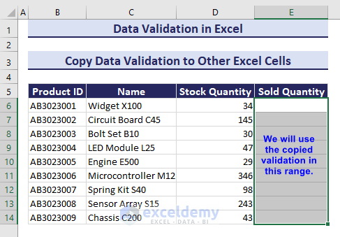
- Select any cell in “Stock Quantity”.
- Press Ctrl + C.
- Select all the cells in the column “Sold Quantity”.
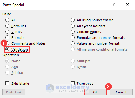
- Right-click, then click on Paste Special from the menu.
- Click on Validation under Paste and choose OK.
- If you enter the number in the cell of “Sold Quantity”, it will allow it. But if you enter any text, an error message box will pop up.
- You can enter the numbers in the cells of the column.
How to Find Cells Containing Data Validation Rules
In the image below, we have a dataset that contains Data Validation, but we don’t know in which column.
- Click on Home and go to Find & Select.
- Choose Data Validation from the list.
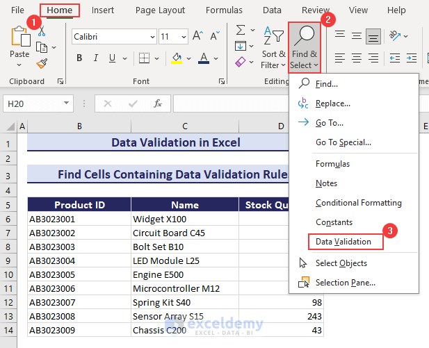
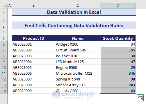
- This will select the column or cells that contain Data Validation. (i.e., D6:D16).
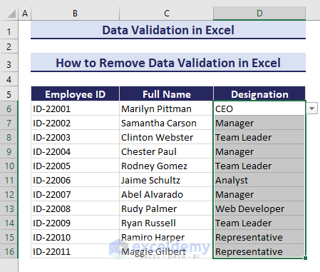
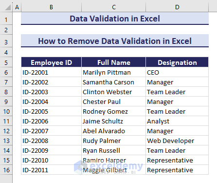
How to Remove Data Validation in Excel
We have a dataset below that contains Data Validation in the “Designation” column. Let’s remove it.
- Select the range D6:D16 in the column.
- Click on Data and go to Data Validation.
- Click on “Clear All” in the Data Validation dialogue box.
- Select OK.
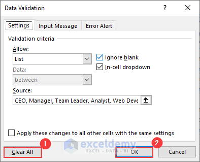
- This will remove the existing Data Validation in the selected cells.
Useful Tips to Apply Data Validation in Excel
- Use dropdowns for consistent and error-free entries.
- Provide informative messages for user guidance.
- Configure alerts for invalid entries.
- Use named ranges for flexible dropdowns.
- Employ formulas for specific validations.
- Consider protecting sheets to enforce rules.
- Thoroughly test before finalizing rules.
What Are the Limitations of Data Validation in Excel?
- Errors are detected only after moving to the next cell.
- Rules need to be set up individually for each sheet.
- Rules apply at the cell level, not across multiple cells.
- Dropdowns don’t automatically update if the source list changes.
- Built-in date range options are somewhat limited.
- Customization options for error alerts are limited.
- No built-in option to restrict or allow specific special characters.
Issues with Data Validation and How to Solve Them
There are some other issues like Data Validation not working properly for Copy&Paste, and Data Validation Greyed out in Excel. You can go through the articles to learn about these common issues and learn how to fix them.
Download the Practice Workbook
Data Validation in Excel: Knowledge Hub
- How to Set Limit in Excel Cell
- Excel Formula Not to Exceed a Certain Value
- Data Validation List from Table in Excel
- Data Validation List from Another Sheet
- Excel Data Validation for Date Format
- How to Use Data Validation in Excel with Color
- Circle Invalid Data in Excel
- Data Validation with Checkbox Control in Excel
- [Fixed] Data Validation Not Working for Copy Paste in Excel
- Excel Data Validation Greyed Out
- Multiple Data Validation in One Cell
- How to Copy Data Validation in Excel
- Remove Blanks from Data Validation List in Excel
- Remove Data Validation Restrictions in Excel
- Excel Custom Data Validation
<< Go Back to Learn Excel
Get FREE Advanced Excel Exercises with Solutions!
