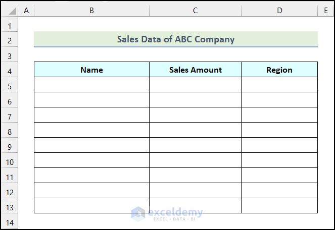
Scenario
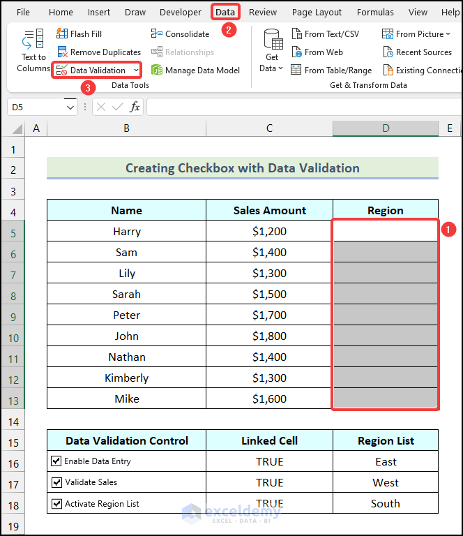
Imagine we have an empty dataset for ABC Company’s sales data. Our objective is to populate this dataset using data validation with checkbox controls.
Here’s a brief overview of how we’ll accomplish this:
- In the Name column, we’ll accept only text input.
- For the Sales Amount column, only numerical inputs will be allowed.
- The Region column will use a drop-down list to fill in the cells.
- Across all columns, checkboxes must be activated; otherwise, data cannot be inserted.
Step 1 – Inserting Checkboxes
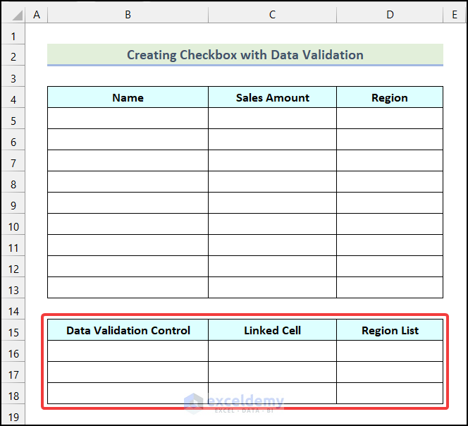
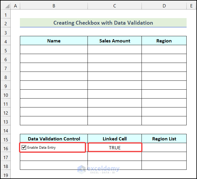
- Create the table as shown in the below image.
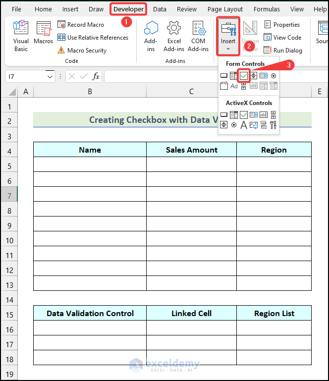
- Go to the Developer tab in the Ribbon.
- Click on Insert in the Controls group.
- Choose Check Box (Form Control) from the dropdown.
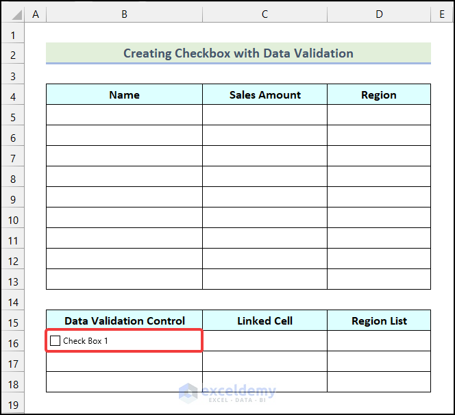
- Draw a checkbox in the Data Validation Control column as shown below.
- Right-click on the checkbox and select Edit Text.
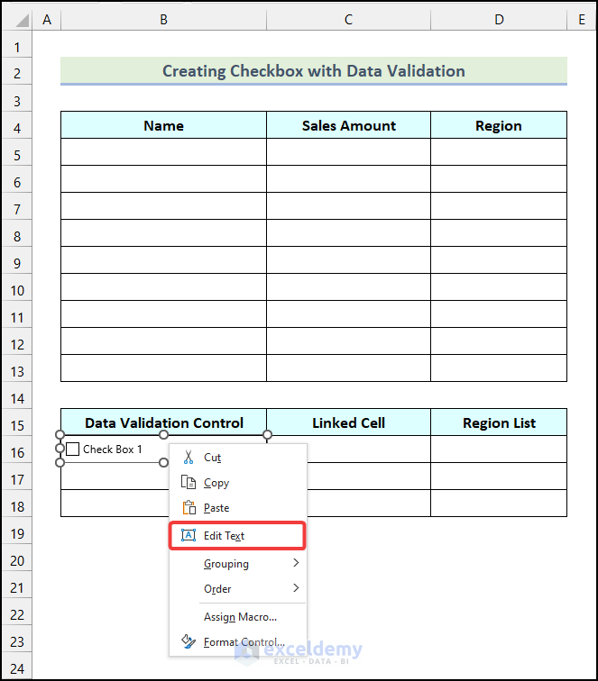
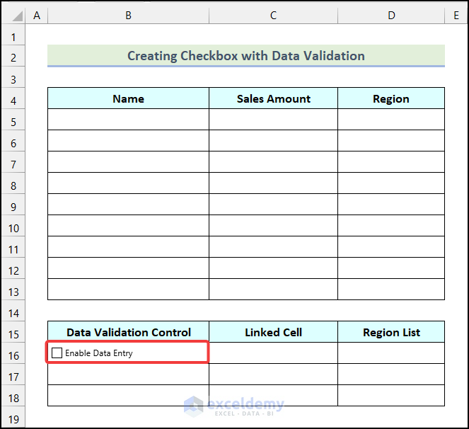
- Rename the checkbox (e.g., Enable Data Entry).
Step 2 – Linking Checkboxes to Cells
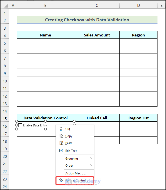
- Right-click on the Checkbox.
- Select Format Control.
- In the Format Control dialog, go to the Control tab.
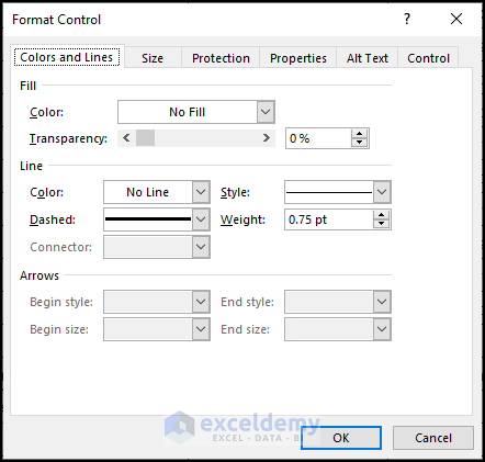
- Choose cell C16 in the Cell link field.
- Click OK.
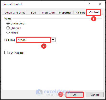
- If you check the Enable Data Entry checkbox, TRUE will appear in cell C16.
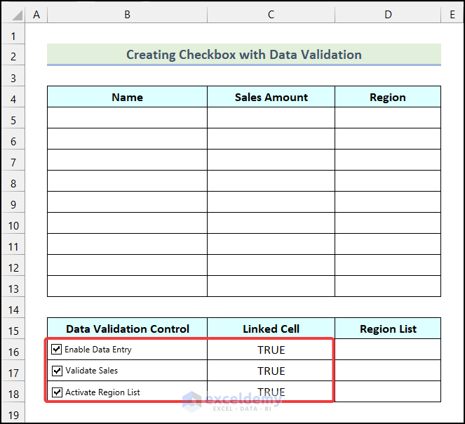
- Follow the same procedure to create two more Checkboxes and link them with cells C17, and C18 respectively.
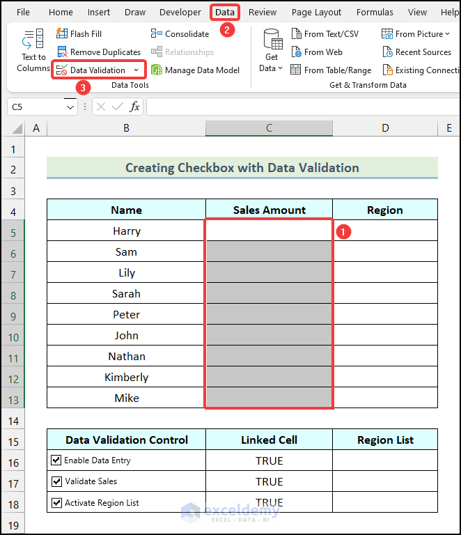
Step 3 – Data Validation for Name Column
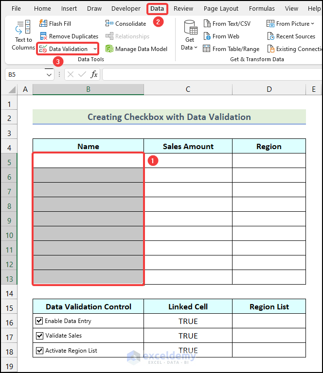
- Select all cells in the Name column.
- Go to the Data tab in the Ribbon.
- Choose Data Validation from the Data Tools group.
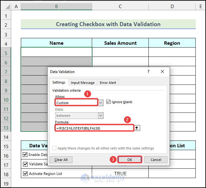
- In the Data Validation dialog, select Custom in the Allow field.
- Enter the following formula in the Formula field:
=IF($C$16,ISTEXT(B5),FALSE)
- Here, cell C16 represents the linked cell, and cell B5 is the first cell in the Name column.
- The formula checks if the value in B5 is text (TRUE) or not (FALSE).
Formula Breakdown
- Here, the ISTEXT function returns a TRUE or FALSE value based on whether the value in cell B5 text or a number is.
- Cell B5 is the value argument.
- Output → TRUE.
- In the IF function,
- $C$15 → This is the logical_test argument.
- ISTEXT(B6) → This refers to the value_if_true argument.
- FALSE → It indicates the value_if_false argument.
- Output → TRUE.
- Click OK.
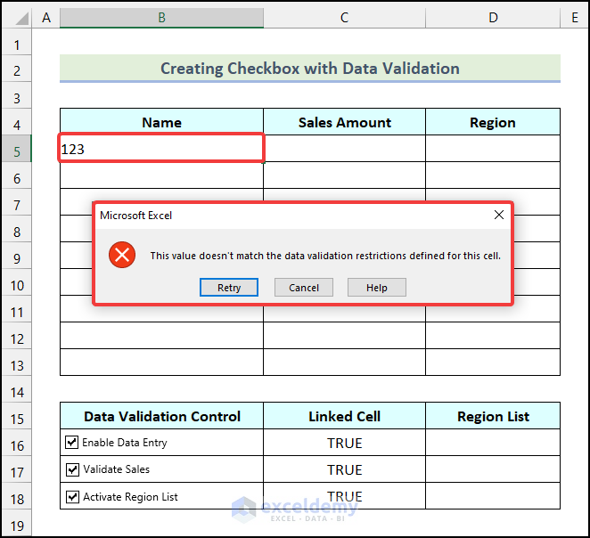
Insert a numerical value in cell B5 (you’ll see an error).
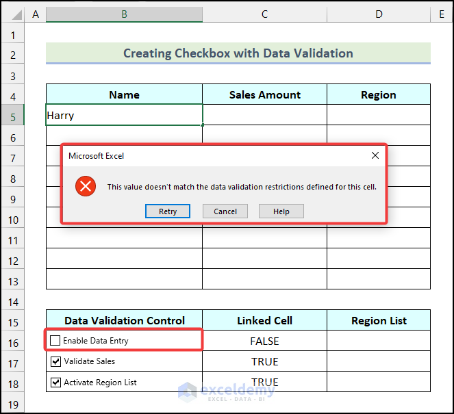
Insert a text value in B5 with the Enable Data Entry checkbox unchecked (another error).
The checkbox ensures that only text values are accepted in the Name column.
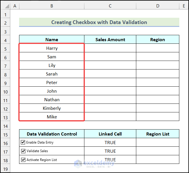
Enter the Name of the salespersons in the Name column while keeping the Enable Data Entry Checkbox checked.
Step 4 – Develop Data Validation for Sales Amount Column
- Highlight/select all the cells in the Sales Amount column.
- Go to the Data tab in the Ribbon.
- Click on Data Validation in the Data Tools group.
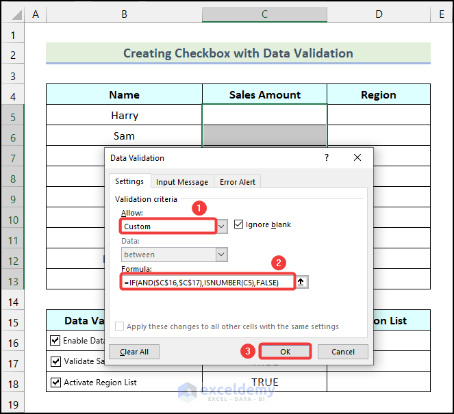
- In the Data Validation dialog, choose Custom in the Allow field.
- Enter the following formula in the Formula field:
=IF(AND($C$16,$C$17),ISNUMBER(C5),FALSE)- Here:
- Cell C17 refers to the second cell of the Linked Cell column.
- Cell C5 represents the first cell of the Sales Amount column.
- The formula checks if the value in C5 is a number (TRUE) or not (FALSE).
Formula Breakdown
- The ISNUMBER function returns a TRUE or FALSE value based on whether a value is a number or a text.
- Here, cell C5 is the value argument.
- Output → TRUE.
- In the AND function,
- $C$16 → It is the logical1 argument.
- $C$17 → This refers to the [logical2] argument.
- Output → TRUE.
- The IF function becomes → IF(TRUE,TRUE,FALSE).
- Output → TRUE.
- Click OK.
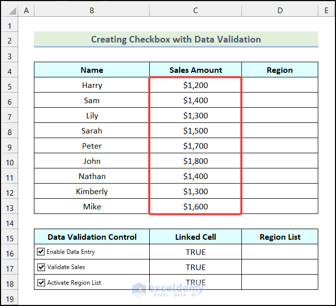
- Ensure that both the Enable Data Entry and Validate Sales checkboxes are checked.
- Enter the Sales Amount for each salesperson.
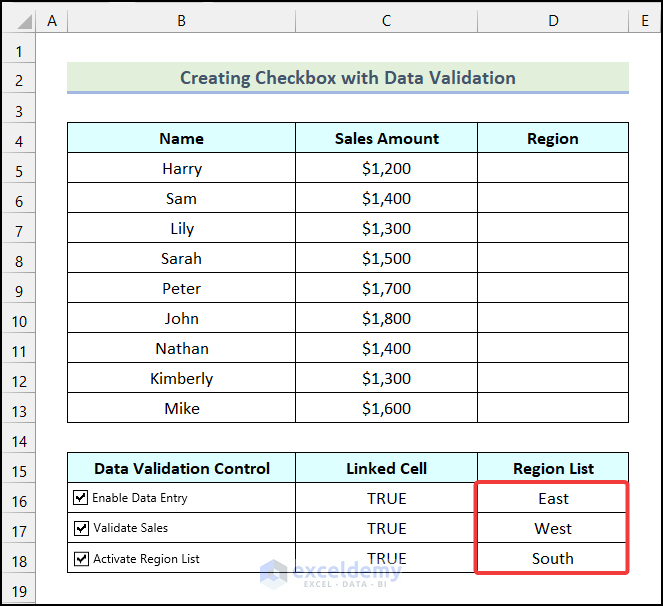
Step 5 – Constructing a Drop-Down List for the Region Column
- In the Region List column, insert the available Regions as shown in the image below (e.g., East, West, South).
- Highlight all the cells in the Region column.
- Go to the Data tab from Ribbon.
- Select the Data Validation option from the Data Tools group.
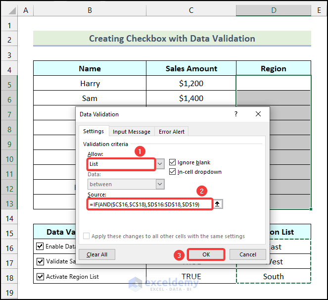
- In the Data Validation dialogue box, select the List option in the Allow field.
- Enter the following formula in the Source field:
=IF(AND($C$16,$C$18),$D$16:$D$18,$D$19)- Here:
- Cell C18 refers to the third cell of the Linked Cell column.
- The range D16:D18 represents the cells of the Region List column.
- Cell D19 represents a blank cell.
Formula Breakdown
- Here, in the AND function,
- $C$16 → It is the logical1 argument.
- $C$18 → This refers to the [logical2] argument.
- Output → TRUE.
- The IF function becomes → IF(TRUE,$D$16:$D$18,$D$19).
- Here, TRUE → This is the logical_test argument.
- $D$16:$D$18 → It refers to the value_if_true argument.
- $D$19 → This indicates the value_if_false argument.
- Output → {“East”;”West”;”South”}.
- Click OK.
Result:
-
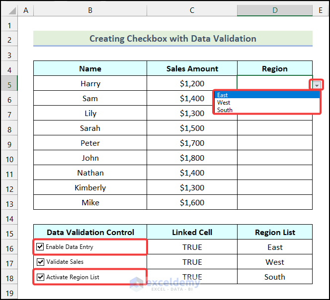
- Drop-down icons will appear in each cell of the Region column.
- Make sure both the “Enable Data Entry” and “Activate Region List” checkboxes are checked.
- Click the drop-down icon next to cell D5 to access the region list.
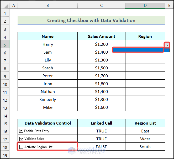
If you uncheck any of the previously mentioned Checkboxes, the drop-down list will disappear.
- Insert the Regions for respective salespersons in the Region column, as demonstrated in the image below.
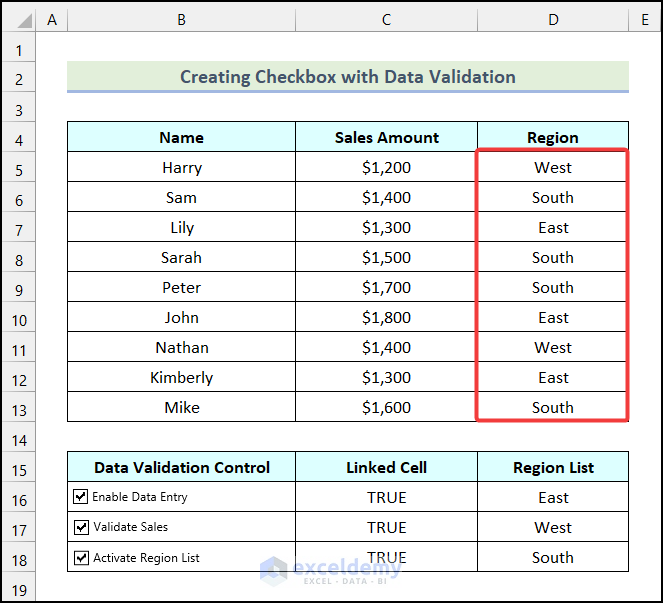
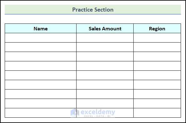
Practice Section
In the Excel Workbook, we have provided a Practice Section on the right side of the worksheet.
Download Practice Workbook
You can download the practice workbook from here:
Related Articles
- How to Perform Data Validation for Alphanumeric Only in Excel
- Excel Data Validation for Date Format
- How to Use Data Validation in Excel with Color
- How to Circle Invalid Data in Excel
- [Fixed] Data Validation Not Working for Copy Paste in Excel
- Excel Data Validation Greyed Out
<< Go Back to Data Validation in Excel | Learn Excel
Get FREE Advanced Excel Exercises with Solutions!
