How to Apply Multiple Data Validation in One Cell in Excel: 3 Methods

Method 1 – Apply Multiple Data Validation in One Cell in Excel with Specific Criteria

STEPS:

Combine the criteria formulas in a nested formula in cell C13. Copy the nested formula from the formula bar but do not paste it anywhere.

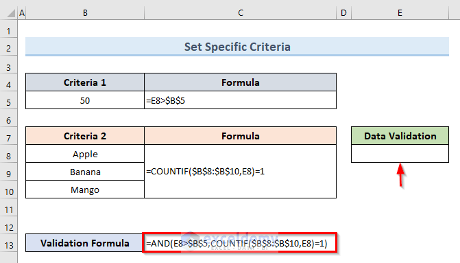
Select cell E8.
Go to Data > Data Tools > Data Validation > Data Validation.

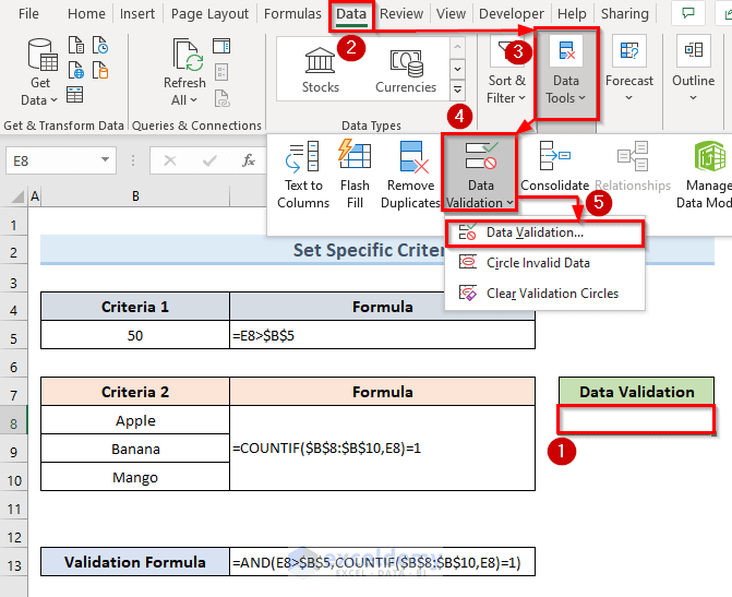
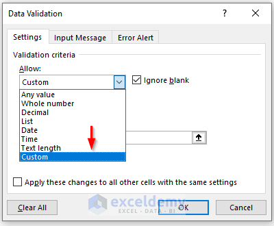
The above action will open a new dialogue box named Data Validation.
Select the option Custom from the Allow drop-down menu.

Paste the validation formula in the Formula text box:

=AND(E8>$B$5,COUNTIF($B$8:$B$10,E8)=1)

Click OK.

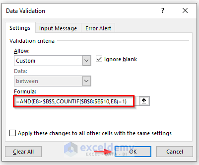
The COUNTIF function checks if the input value matches with the range values (B8:B10). The AND function combines the two criteria.

Input value 40 in cell E8.

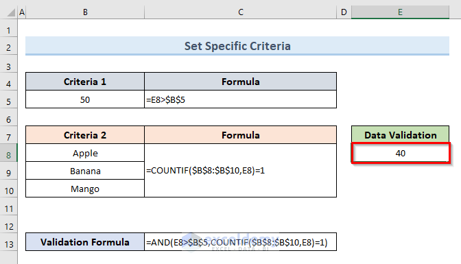
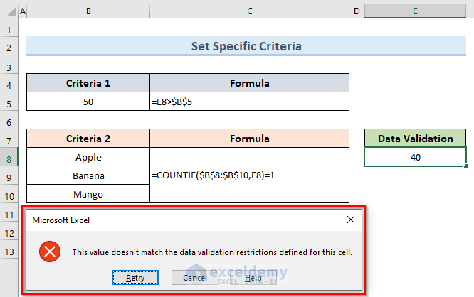
Excel will give us a warning prompt box for the above value as it doesn’t match our ‘Criteria 1’. The value in cell E8 must be greater than 50.

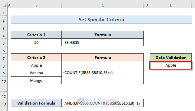
Enter the text ‘Apple’ in cell E8. This value meets the second criterion as it is in the range (B8:B10).

Method 2 – Allow a Text and a Date between Two Dates by Applying Multiple Data Validation in One Cell

STEPS:

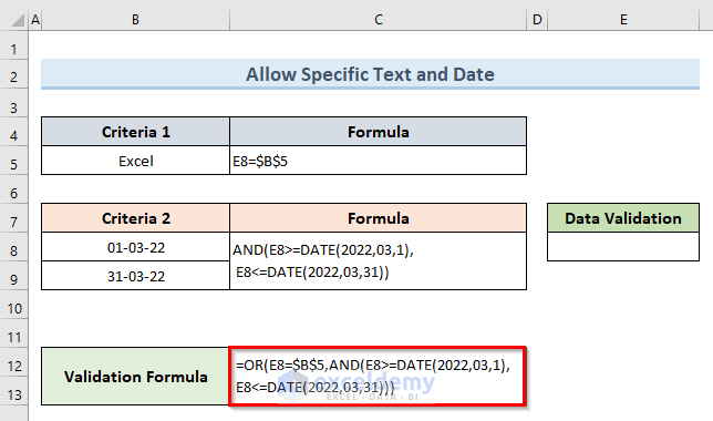
Merge the criteria formulas in a nested formula with the AND function in cell C12.
Copy the nested formula from the formula bar but don’t paste it anywhere.

Open the data validation window.
Select the option Custom from the Allow drop-down. Insert the validation formula in the Formula text box:

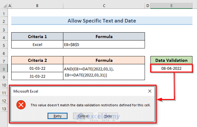
=OR(E8=$B$5,AND(E8>=DATE(2022,03,1),E8<=DATE(2022,03,31)))

Click OK.

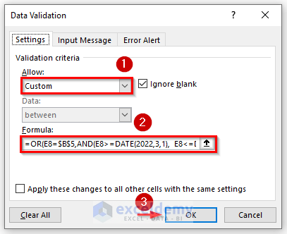
The AND function checks if the input date is between ‘1-03-22’ & ‘31-03-22’. The OR function combines the two criteria and gives output if anyone is true.

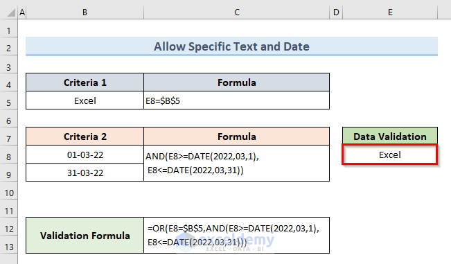
Enter the text Excel in cell E8, because it matches the ‘Criteria 1’ of our data validation formula.

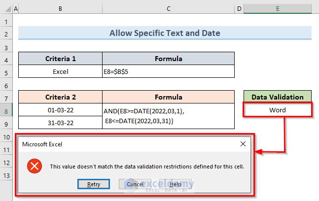
Input the text Word in cell E8, it will show a warning prompt box. It’s happening because the text value Word doesn’t match any criteria.

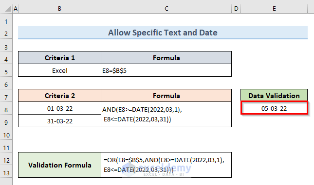
A date in cell E8 which from the date range ‘1-03-22’ to ‘31-03-22’. Excel accepts the value as it matches with ‘Criteria 2’.

Write a date in cell E8 outside the date range of the validation formula. Excel gives a warning prompt box that the given value doesn’t match any criteria of our validation formula.

Method 3 – Use Multiple Data Validation in One Cell in Excel to Fix Starting Character and Length of a String

STEPS:

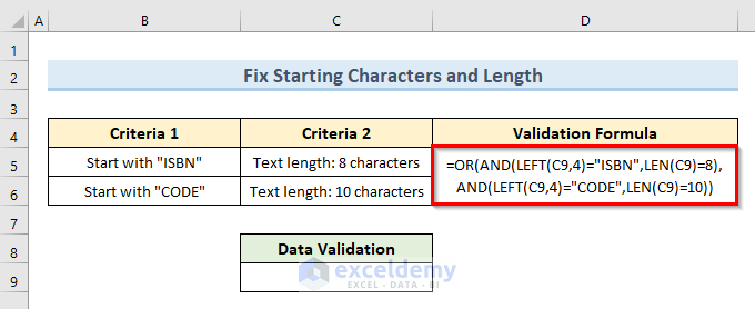
Create the data validation formula in cell D5 that covers all the criteria.

Open the Data Validation dialogue box like the example-1. Select the option Custom from the Allow drop-down menu.
Insert the data validation formula in the Formula text box.

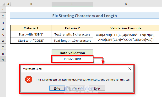
=OR(AND(LEFT(C9,4)="ISBN",LEN(C9)=8),AND(LEFT(C9,4)="CODE",LEN(C9)=10))

Click OK.

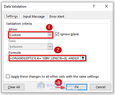
The LEFT function extracts 4 characters from the string. The LEN function calculates the length of the string. The OR function combines the two criteria and gives output if anyone is true.

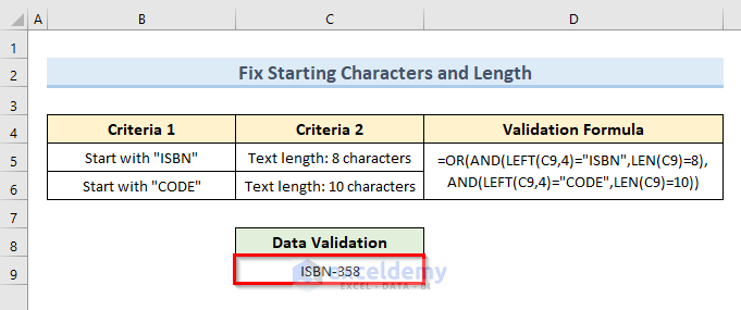
Insert the value ‘ISBN-358’. The value starts with characters ‘ISBN’ and the length of the string is 8. Excel accepts the value as it matches both criteria.

Add two more characters with the previous input value. Excel shows a warning prompt box, though it starts with the text ‘ISBN’, which matches the first criteria. But the text contains 10 characters that don’t match the second criteria.