How to Use IF Statement in Data Validation Formula in Excel (6 Ways)

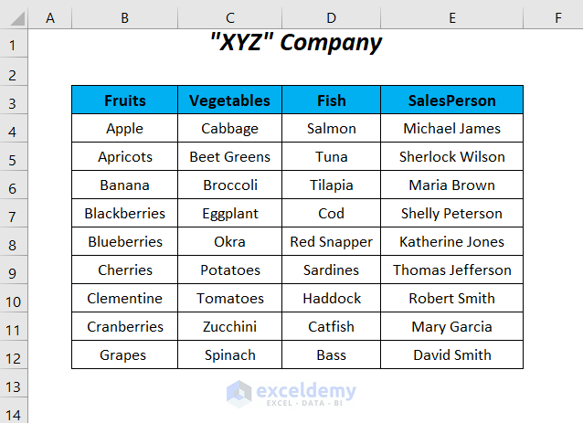
Here, we have some records of some of the products and their corresponding salesperson’s names of a company. By using this dataset, we will demonstrate how to use the IF statement in the Data Validation formula in Excel.

Method 1 – Using IF Statement to Create a Conditional List with the Help of Data Validation Formula

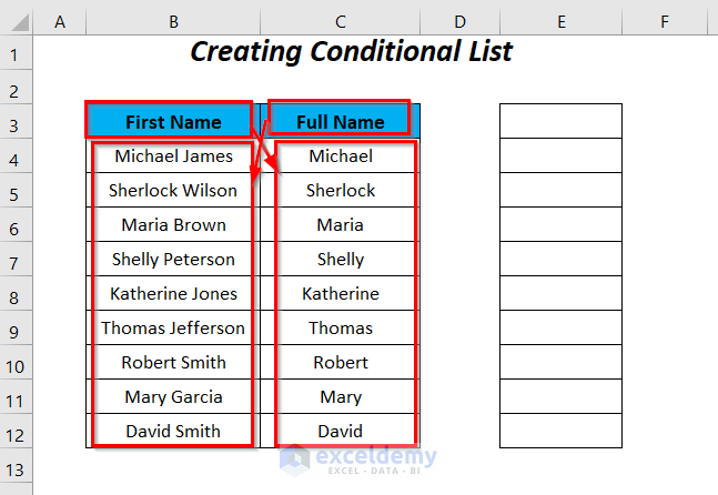
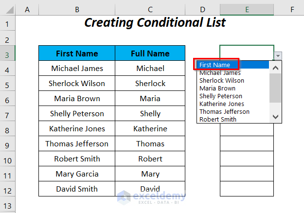
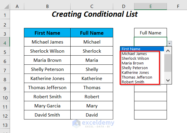
For this method we have arranged the full names of the employees under the header First Name and for the first name of the employees, we have used the header Full Name. Using the IF function in the data validation formula we will make the conditional list in the right-side table.

Steps:

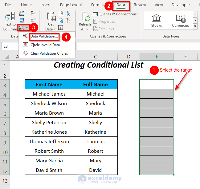
• Select the range E3:E12.
• Go to the Data tab and the Data Tools group.
• Select the Data Validation dropdown.
• Choose the Data Validation option.

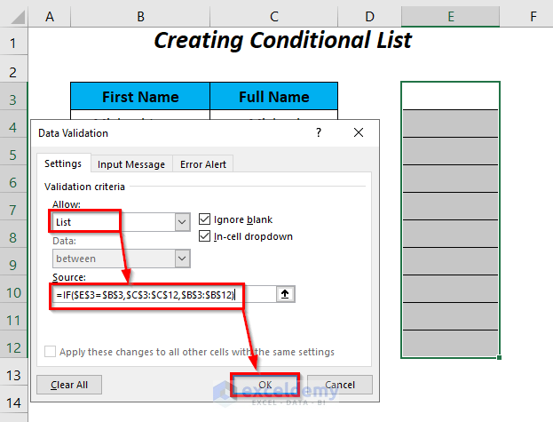
Then, the Data Validation dialog box will appear.

• Select the List option in the Allow box.
• Write the following formula in the Source box and click OK:

Here, $E$3 is the cell where we want to select the header from the dropdown list and $B$3 is the header name of the first column. When these two values are equal, the IF function will return the list of the range $C$3:$C$12, otherwise the list will contain the values of the range $B$3:$B$12.

• When we click on the drop-down symbol of cell E3, we will get the header First Name.

• Select the first names from the list of the first names of cell E4.

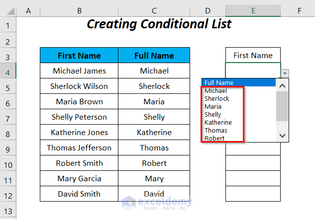
In this way, we are getting the first names of the salesperson’s names along with the header First Name.

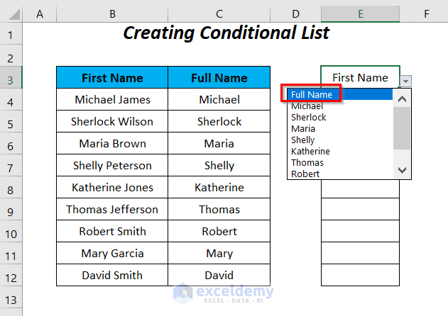
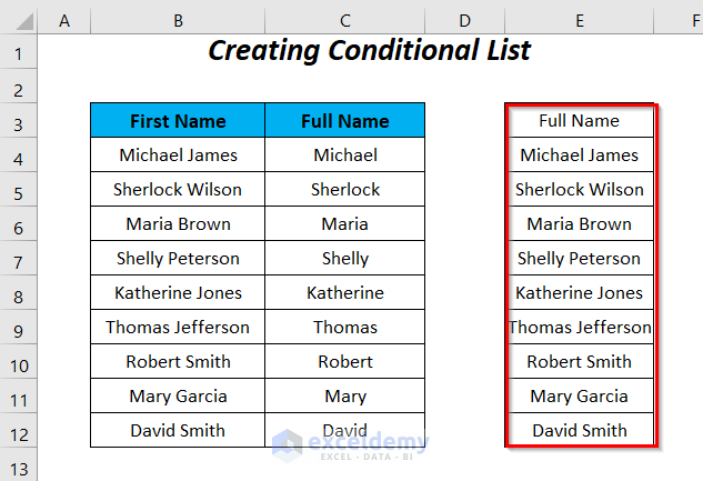
• You can change the header name from First Name to Full Name in cell E3.

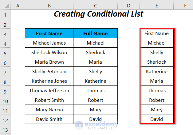
• Select the full names from the list for the rest of the cells.

You will get the full names of the employees with the corresponding header.

Read More: How to Use Custom VLOOKUP Formula in Excel Data Validation

Method 2 – Creating a Dependent Dropdown List by Using IF Statement in Data Validation Formula

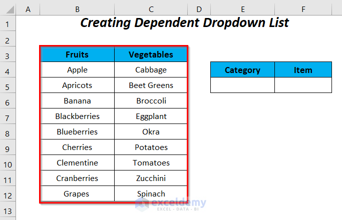
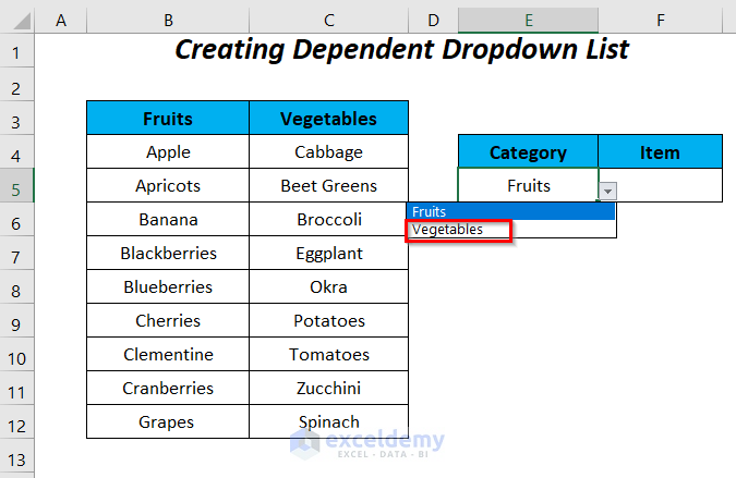
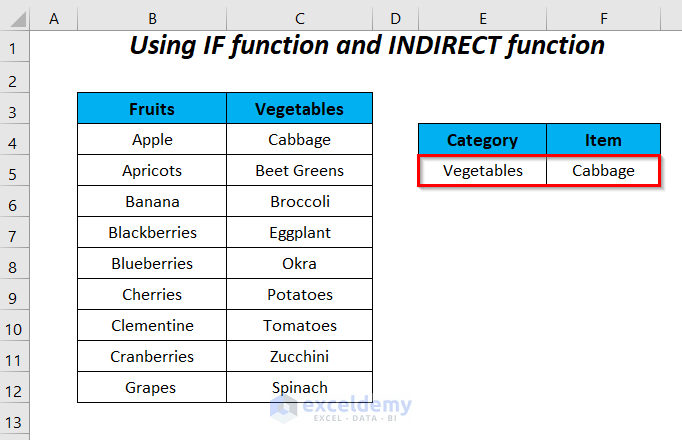
In this section, we will create a dependent dropdown list where the Item list will be dependent on the Category list.

Steps:

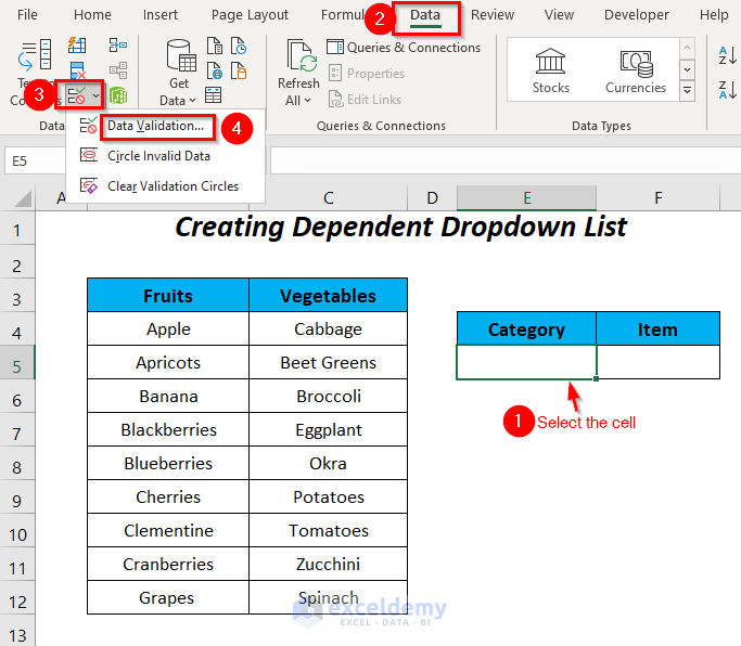
• Select the cell E5 and go to the Data tab.
• In the Data Tools group, go to the Data Validation dropdown and select the Data Validation option.

The Data Validation dialog box will appear.

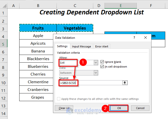
• Select the List option in the Allow box and write the following formula in the Source box:

Here, $B$3 is the header Fruits and $C$3 is the header Vegetables.

Press OK.

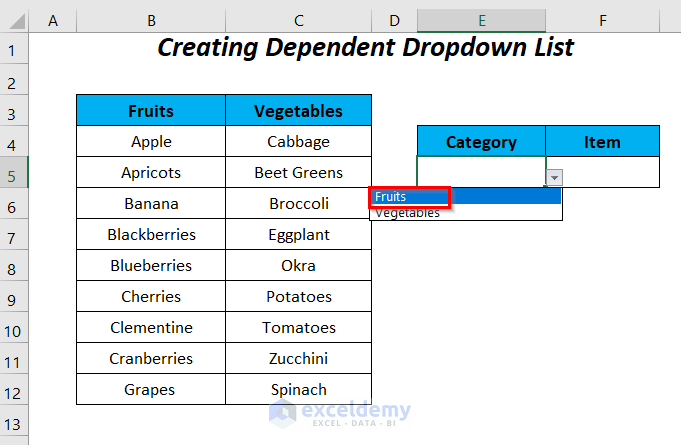
• After clicking the dropdown symbol of cell E5, you will get the header names on the list.
• Let’s select Fruits from this list.

• Select cell F5.
• Choose Data Validation again as for the E5 cell.
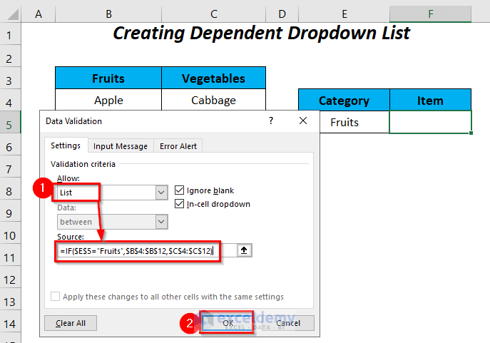
• Select the List option in the Allow box, and write the following formula in the Source box:

When the value of the cell $E$5 will be equal to “Fruits”, IF will return the range $B$4:$B$12 as a list otherwise the list will contain the range $C$4:$C$12.

• Press OK.

• To select a fruit item like Apple, click on the dropdown list of cell F5 and select it from the list.

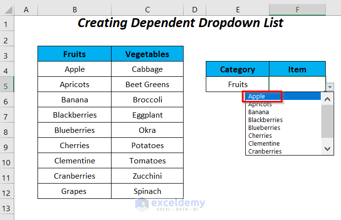
You will get your desired item Apple for the category Fruits.

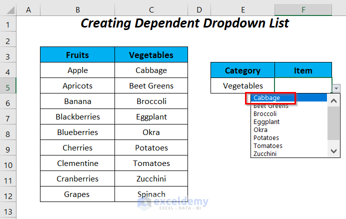
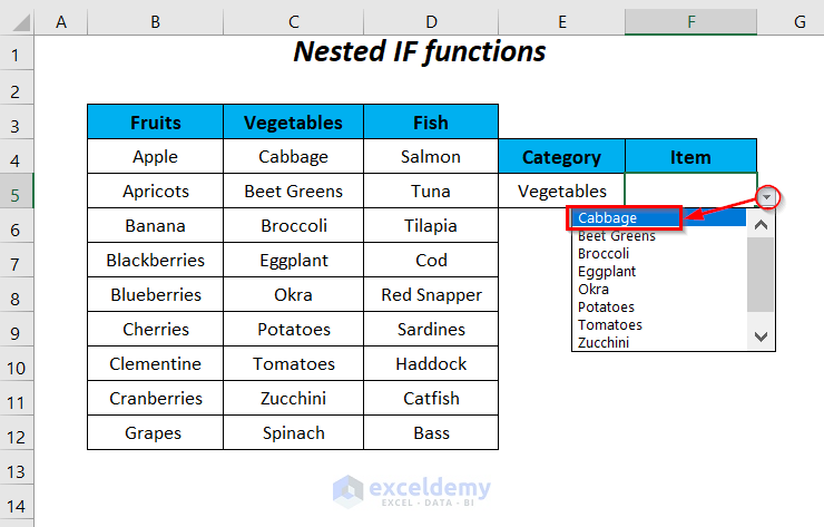
• You can select the Category as Vegetables from the list.

• You will get the list of vegetables in the item list, where you can select one.

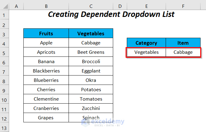
Finally, we are getting the Item Cabbage for the corresponding Category Vegetables.

Read More: Data Validation Based on Another Cell in Excel

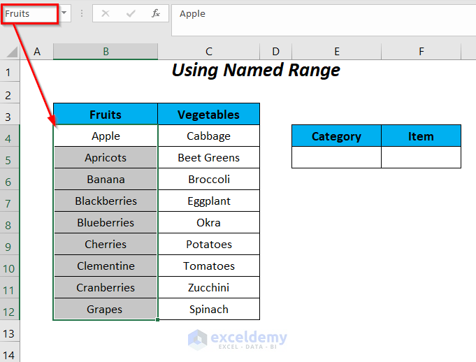
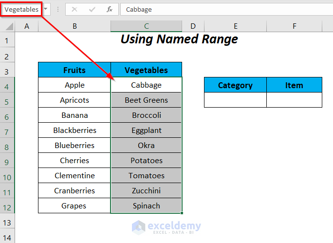
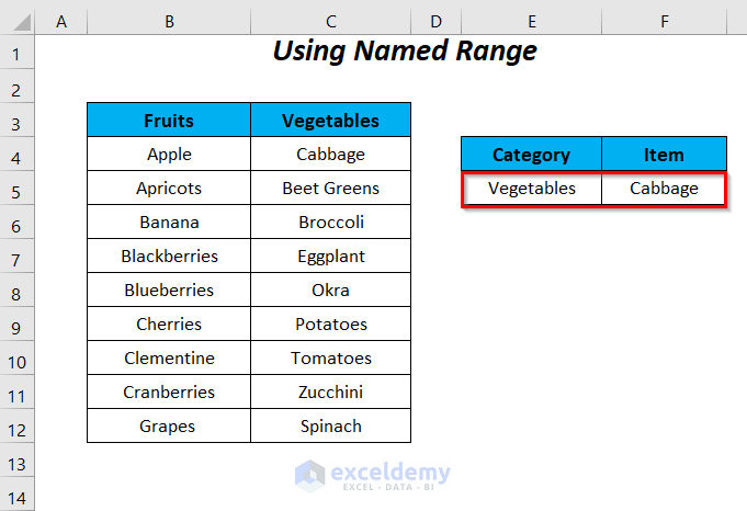
Method 3 – Using IF Statement and Named Range in Data Validation Formula in Excel

For this, we have named the range of fruits as Fruits and the range of vegetables as Vegetables.

Steps:

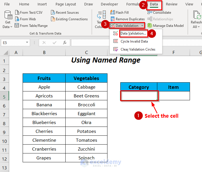
• Select the cell E5.
• Go to the Data tab and, in the Data Tools Group, select the Data Validation dropdown and choose the Data Validation option.

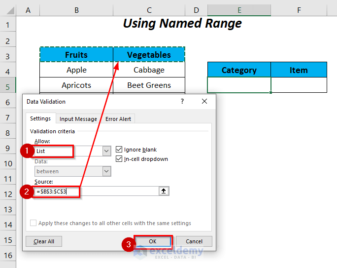
Afterward, the Data Validation dialog box will appear.

• Select the List option in the Allow box and write the following formula in the Source box:

Here, $B$3 is the header Fruits and $C$3 is the header Vegetables.

• Press OK.

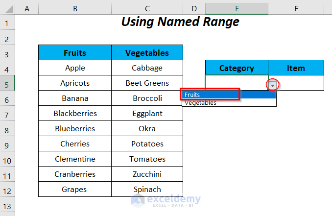
• Click on the dropdown symbol of cell E5 and select Fruits from this list.

Now, it’s time to make the items list in cell F5.

• Select F5.
• Go to the Data tab and, in the Data Tools Group, select the Data Validation dropdown and choose the Data Validation option.
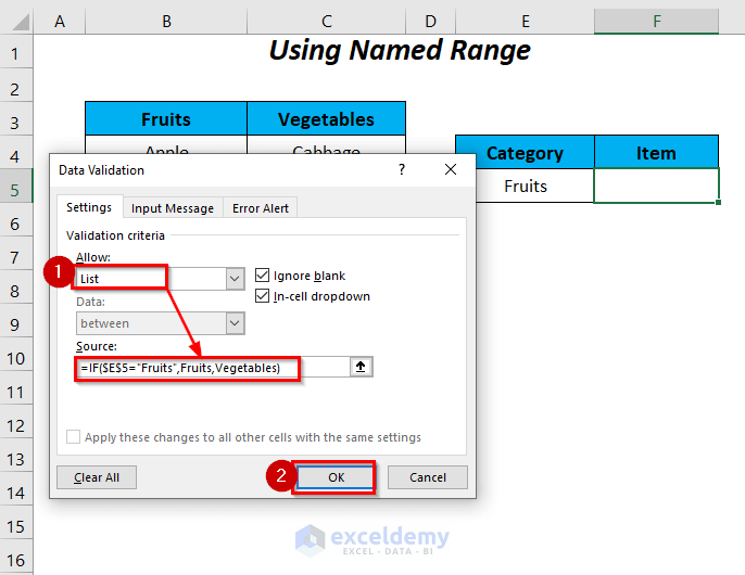
• Select the List option in the Allow box and write the following formula in the Source box:

When the value of the cell $E$5 is equal to “Fruits”, IF will return the named range Fruits as a list otherwise the list will contain the named range Vegetables.

• Press OK.

• Click on the dropdown list of cell F5 and select the item Apple from the list.

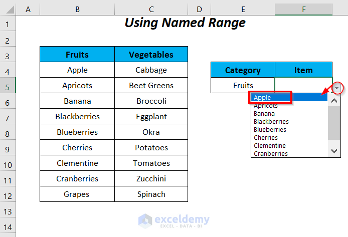
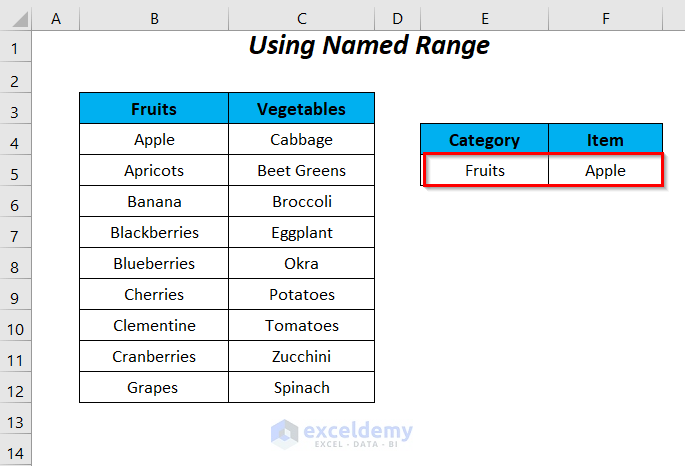
Then, you will get your desired item Apple for the category Fruits.

• Select the item Cabbage from the list for the category Vegetables.

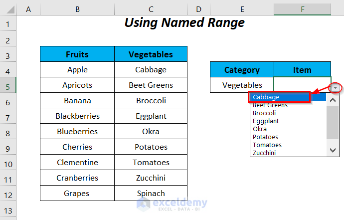
Eventually, we will get the Item Cabbage for the corresponding Category Vegetables.

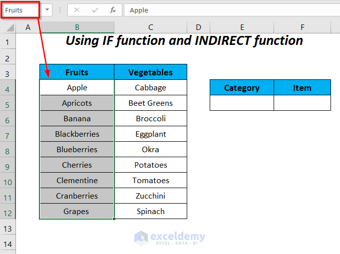
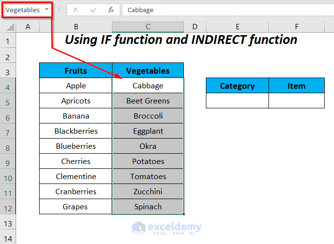
Method 4 – Using the IF and INDIRECT Functions in Data Validation Formula in Excel

We have the following named ranges Fruits and Vegetables for the fruits range and vegetables range respectively.

Steps:

• Select the cell F5.
• Go to the Data tab and, in the Data Tools Group, select the Data Validation dropdown and choose the Data Validation option.

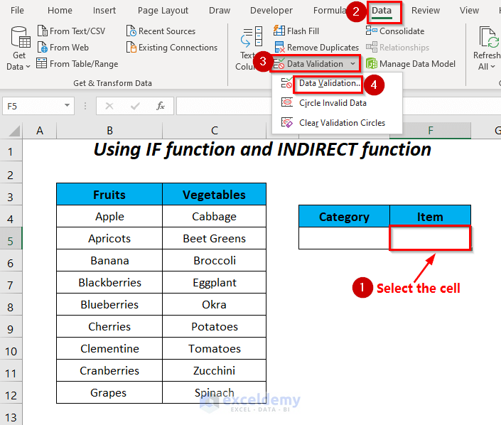
After that, the Data Validation dialog box will appear.

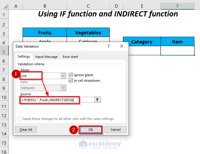
• Select the List option in the Allow box and write the following formula in the Source box:

When the value of the cell $E$5 is equal to Blank, IF will return the named range Fruits as a list otherwise INDIRECT($E$5) will check the value in the cell $E$5 and then link the value as a reference to the corresponding named range.

• Press OK.

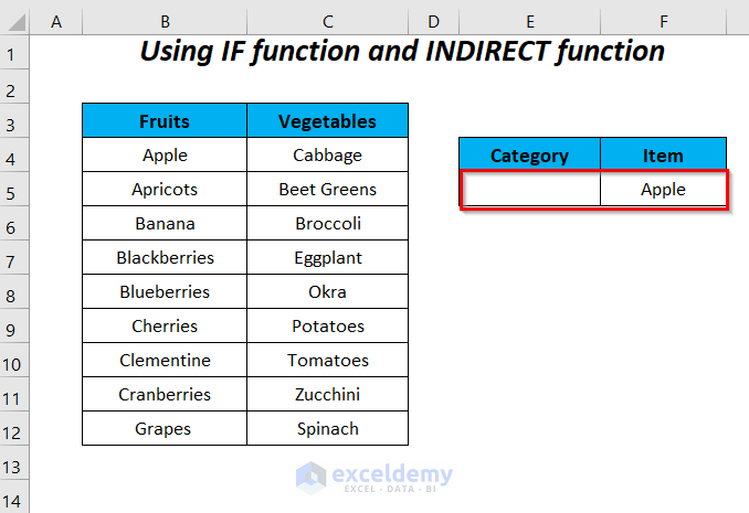
Here, we have a blank in cell E5, and for this blank, we have the list of fruits in the dropdown list of cell F5, and then select the first Apple from the list.

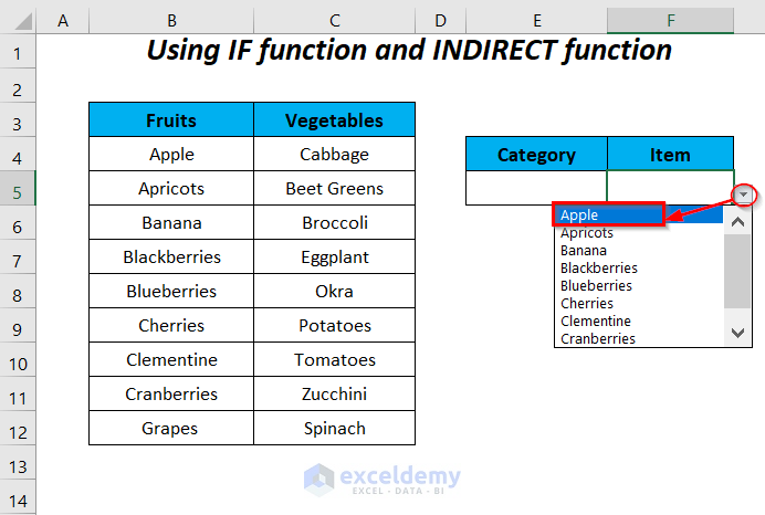
For the blank as a Category, we have the Item as a fruit Apple.

• Write down Vegetables in E5 and then you will get the list of vegetables in cell F5.
• Select Cabbage from the vegetable list of the Item column.

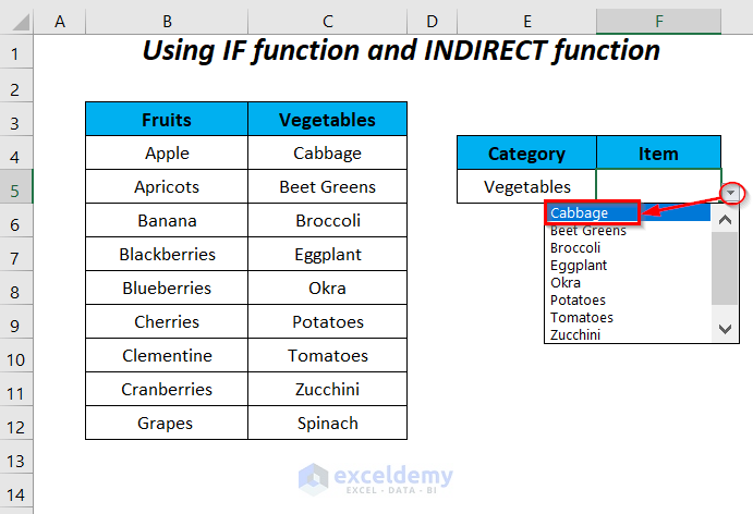
We will get the Item Cabbage for the corresponding Category Vegetables.

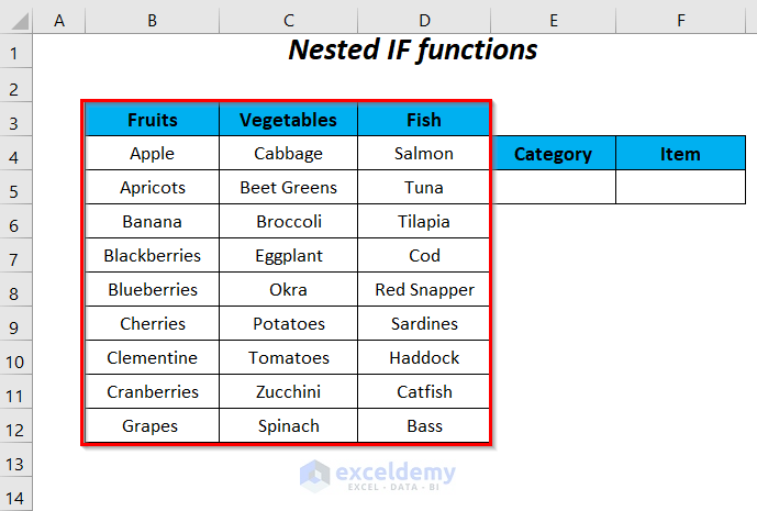
Method 5 – Using Nested IF Functions in Data Validation Formula

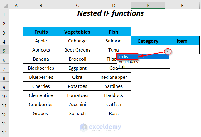
Let’s expand the dataset with Fish.

Steps:

• Select the cell E5.
• In the Data tab, go to the Data Tools Group, select the Data Validation dropdown, and choose the Data Validation option.

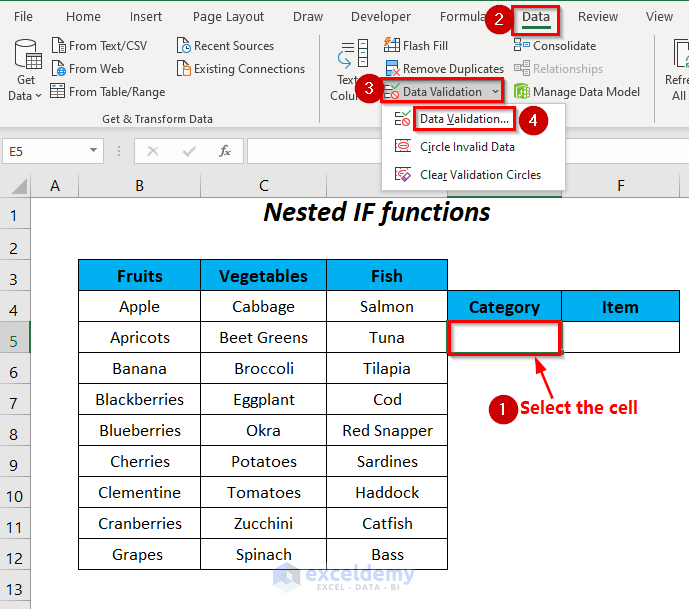
The Data Validation dialog box will appear.

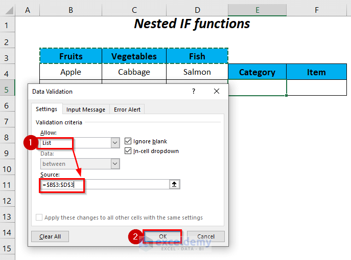
• Select the List option in the Allow box and write the following formula in the Source box:

Here, $B$3 is the header Fruits and $D$3 is the header Fish.

• Press OK.

• Click on the dropdown symbol of cell E5 and select Fruits from this list.

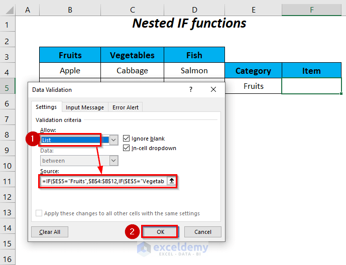
• Select the cell F5.
• In the Data tab, go to the Data Tools Group, select the Data Validation dropdown, and choose the Data Validation option.
• Select the List option in the Allow box and write the following formula in the Source box:

When the value of the cell $E$5 is equal to “Fruits”, IF will return the range $B$4:$B$12 as a list, otherwise it will go to the next IF function which will check for the value “Vegetables”.
If the condition of this function is fulfilled, then it will return the range $C$4:$C$12 as a list otherwise $D$4:$D$12 will be used in the list.

• Press OK.

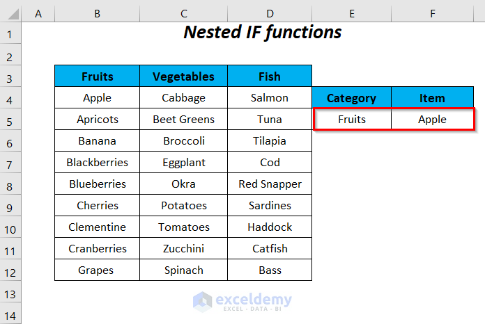
• Click on the dropdown list of cell F5 and select the item Apple from the list.

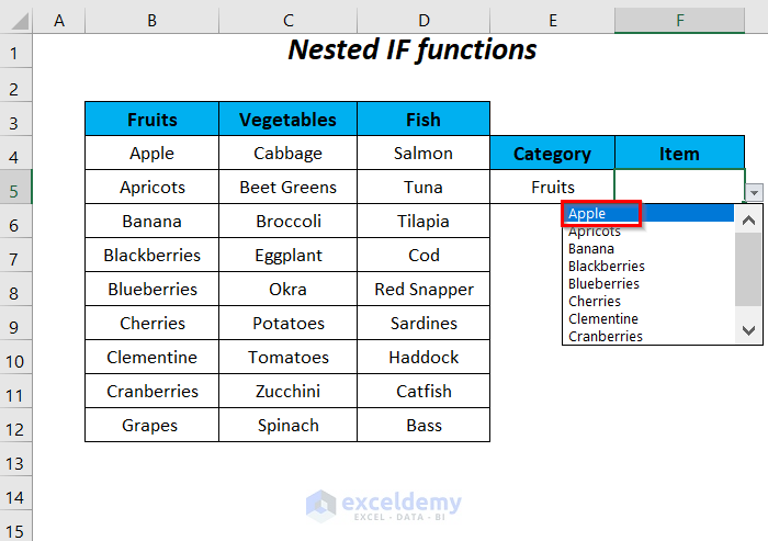
You will get Apple for the category Fruits.

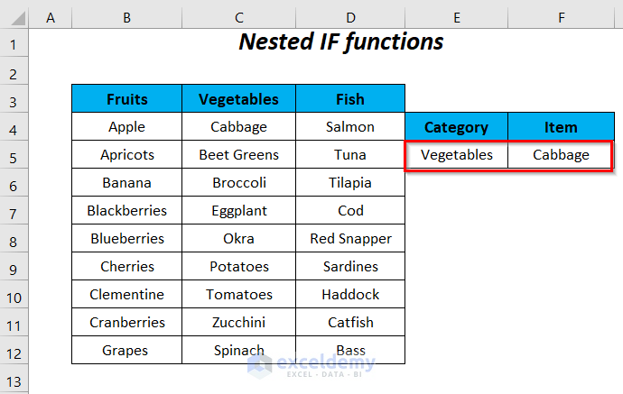
• Select the item Cabbage from the list for the category Vegetables.

Then, you will have the Item Cabbage for the Category Vegetables.

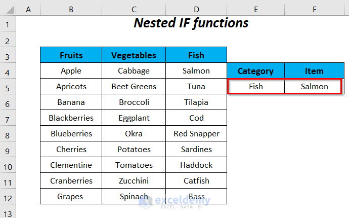
• Select Fish as the category for E5, and then choose an option.

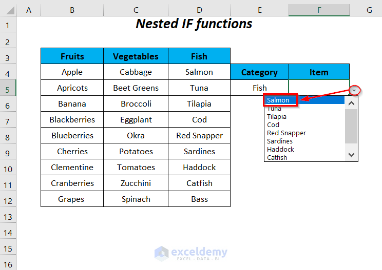
Here’s how you can get Salmon.

Read More: Apply Custom Data Validation for Multiple Criteria in Excel

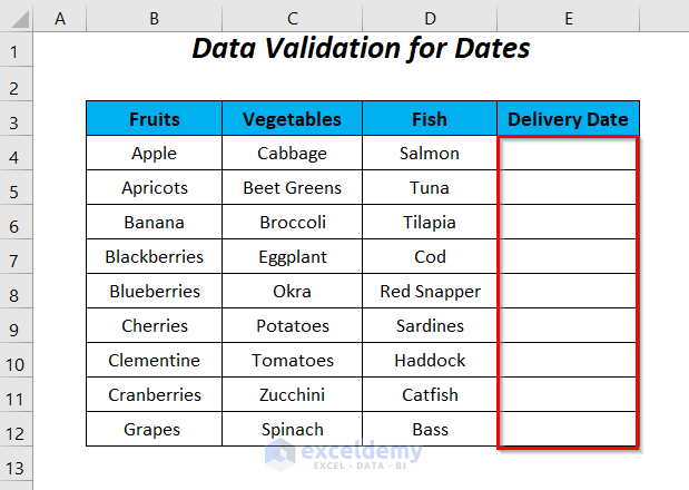
Method 6 – Using IF Statement in Data Validation Formula for Dates

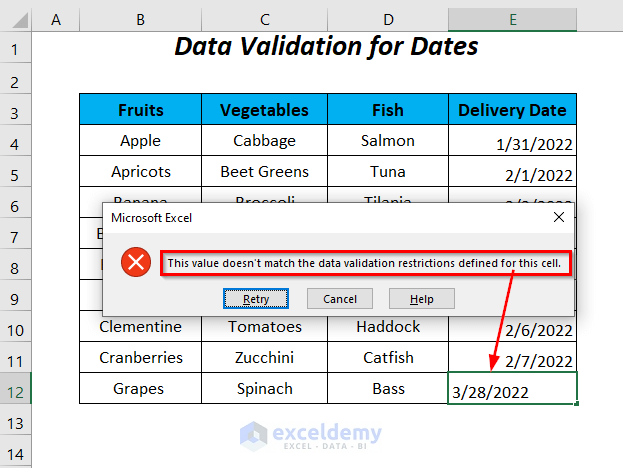
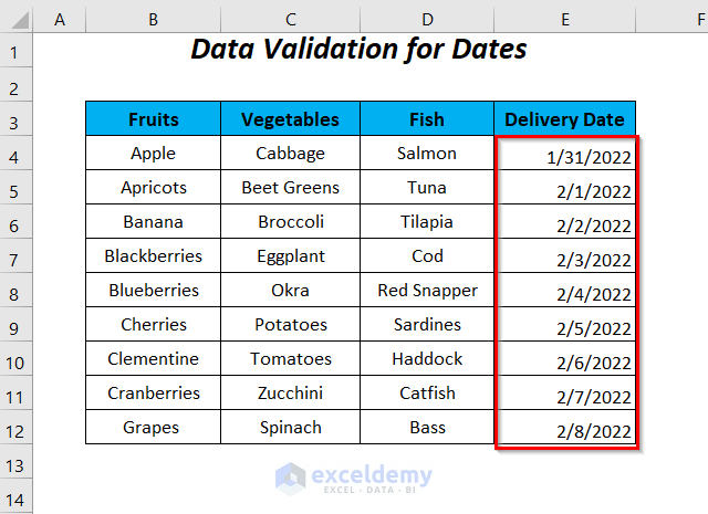
Let’s restrict the entries for the dates of the Delivery Date column in a way that the cells of this column will only accept the dates preceding today’s date (in m/dd/yyyy format), and for entering dates greater than today’s date we will get an error message.

Steps:

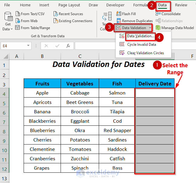
• Select the cell range E4:E12.
• In the Data tab, go to the Data Tools Group, select the Data Validation dropdown, and choose the Data Validation option.

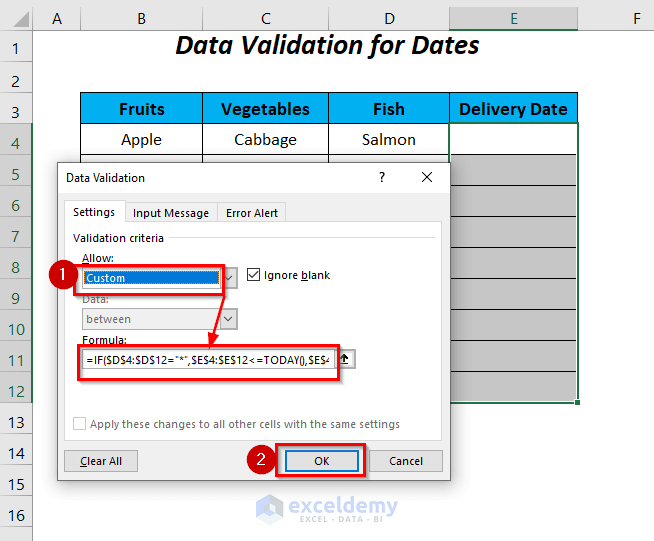
• Select the Custom option in the Allow box and write the following formula in the Source box:

If the cells of the range $D$4:$D$12 contain any text string then the cells of the range $E$4:$E$12 will only allow the dates smaller than today’s date.

• Press OK.

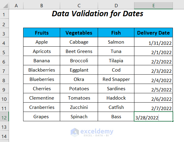
We can enter any date without any problem except for the dates greater than today’s date (written on 2/28/2022).

• Try to enter a date that’s “in the future.”

Excel throws an error message due to the data validation formula set previously.

You can manually fill the cells of the Delivery Date column with dates preceding today.

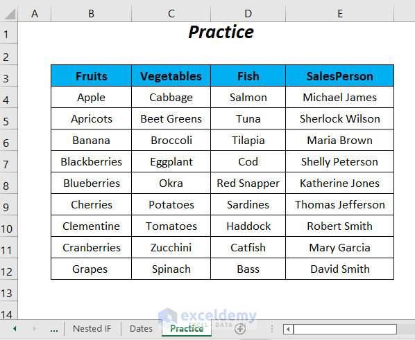
Practice Section

For doing practice by yourself we have provided a Practice section like below in a sheet named Practice. Please do it by yourself.

Download Practice Workbook

Related Articles

• How to Apply Multiple Data Validation in One Cell in Excel
• How to Remove Blanks from Data Validation List in Excel
• How to Remove Data Validation Restrictions in Excel
• How to Copy Data Validation in Excel

<< Go Back to Excel Custom Data Validation | Data Validation in Excel | Learn Excel