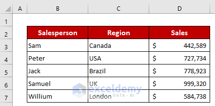
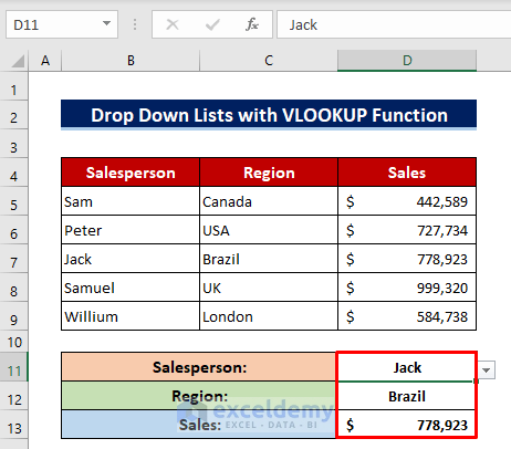
How to Use a Custom VLOOKUP Formula in Excel Data Validation

The sample dataset showcases sales in different regions.

Method 1 – Using a Drop-down List of Data Validation with the VLOOKUP Function in Excel

Steps:

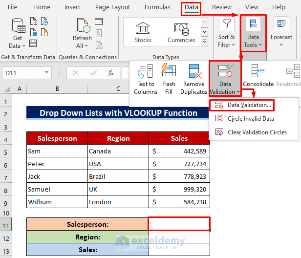
Select D11.
Click: Data > Data Tools > Data Validation > Data Validation.

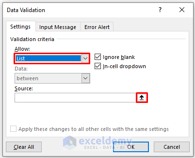
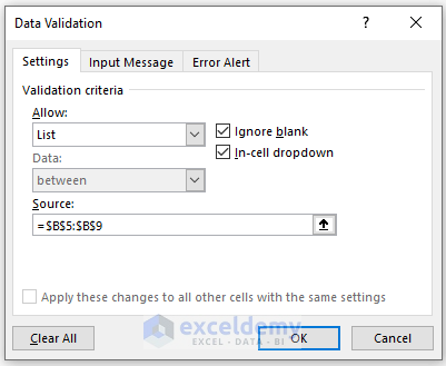
Select Settings.
InAllow, choose List.
In Source, click Open.

Select the salespersons’ names.
Press Enter.

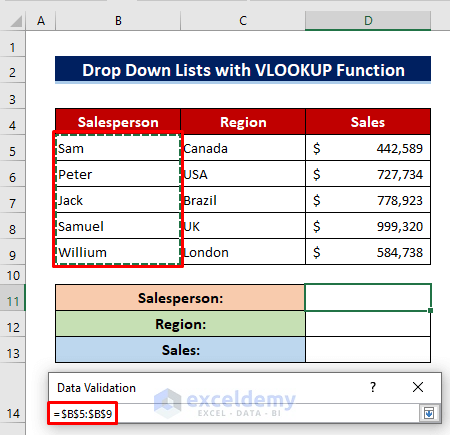
Click OK.

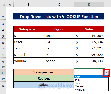
A drop-down icon will be displayed beside the selected cell.
Click it to see the list.
Select Sam and use the VLOOKUP function to find his sales and region.

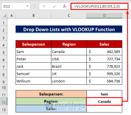
To find the region, enter the following formula in D12:

=VLOOKUP(D11,B5:D9,2,0)

Press Enter to see the output.

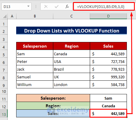
To find the sales in D13:

Enter the following formula.

=VLOOKUP(D11,B5:D9,3,0)

Press Enter to see the output.

Follow the same procedure for the other salespersons.

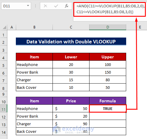
Method 2 – Applying Dynamic Data Validation with a Multiple VLOOKUP Formula

The dataset showcases gadgets and their prices.

Steps:

In D11 enter the following formula:

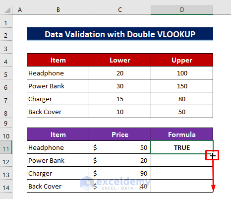
=AND(C11>=VLOOKUP(B11,B5:D8,2,0),C11<=VLOOKUP(B11,B5:D8,3,0))

Press Enter to see the output.

Drag down the Fill Handle to see the other results.

This is the final output:

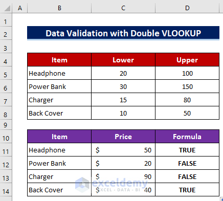
Formula Breakdown:

C11<=VLOOKUP(B11,B5:D8,3,0)
finds the upper range for the value of B11 and checks whether the value of C11 is less than or equal to the output of the VLOOKUP function. It returns TRUE

C11>=VLOOKUP(B11,B5:D8,2,0)
finds the lower range for the value of B11 checks whether the value of C11 is greater than or equal to the output of the VLOOKUP function. It returns TRUE

AND(C11>=VLOOKUP(B11,B5:D8,2,0),C11<=VLOOKUP(B11,B5:D8,3,0))
The AND function combines both outputs. If both return TRUE, it returns TRUE. If one returns FALSE, it returns FALSE.