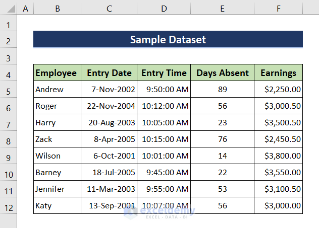
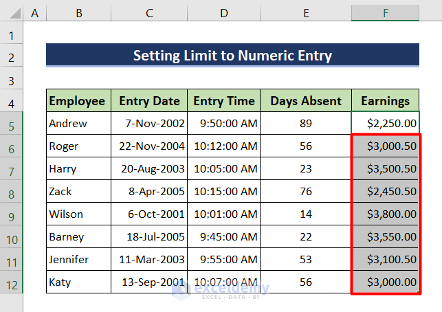
In this article, we will use the following dataset containing various types of cell entries (text, date, time, number and currency) to demonstrate 5 simple ways to set limits in Excel cells.
Method 1 – Setting Limits for Numerical Data Entry
We can limit cells to both whole numbers and decimals.
1.1 – Whole Numbers Only
We can limit cells to Whole Numbers only using the Data Validation tool.
Steps:
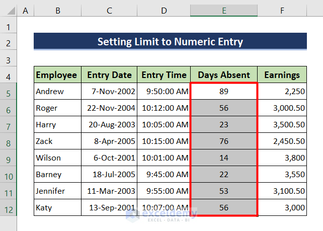
- Select all the data in the Days Absent column.
- Go to the Data tab.
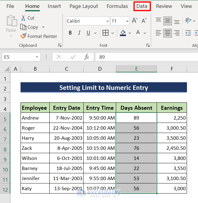
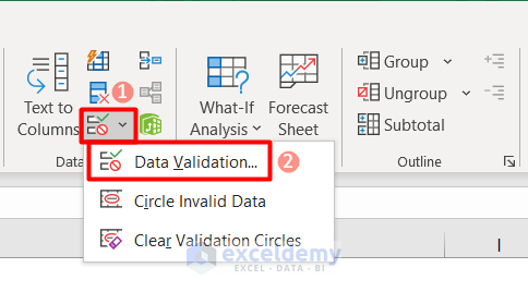
- Click on the Data Validation tool.
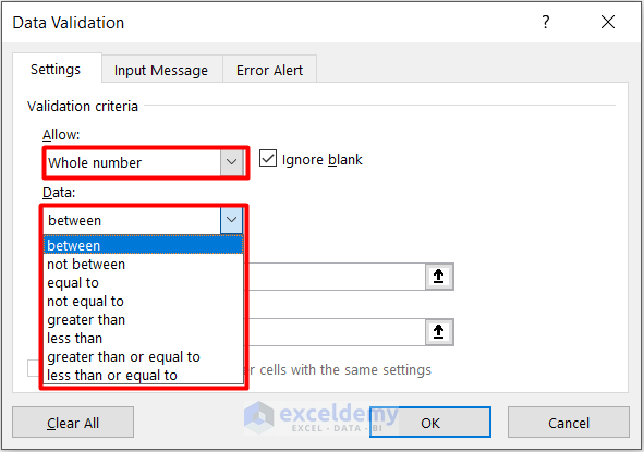
- In the pop-up window that opens, select Whole number in the Allow field.
- In the Data option, select the options set your desired limit or criteria. In this example, we select the between option.
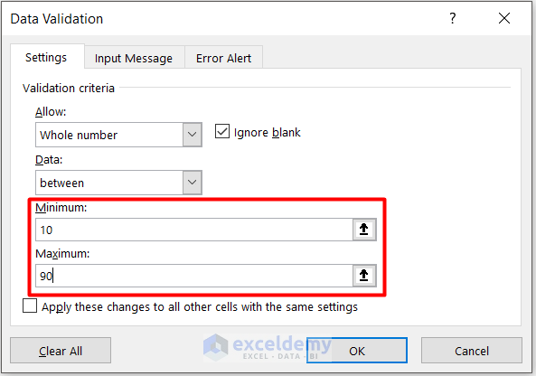
- For the between option, choose minimum and maximum values, here 10 and 90.
Now, this cell will only allow values between 10-90. Any value out of this range will show an error message.
- Click OK.
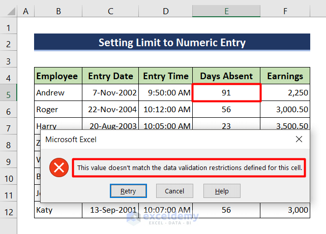
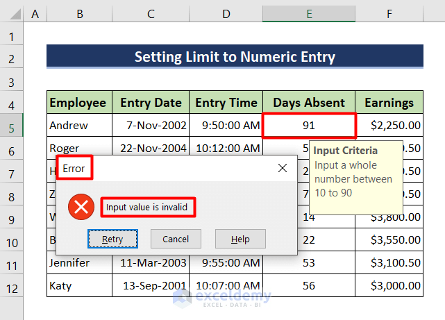
- Try to input a value of more than 90.
We entered 91 in cell E5 and receive a message that this value doesn’t match the criteria.
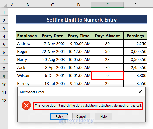
- Try to enter a value less than 10.
We receive the same error message when we try to input 9.
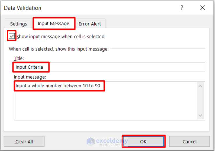
We can modify the error message as well as show input criteria while the cell is selected.
- Click on the Input Message tab in the Data Validation pop-up.
- Change the Title and Input message.
- Make sure that the Show input message box is checked.
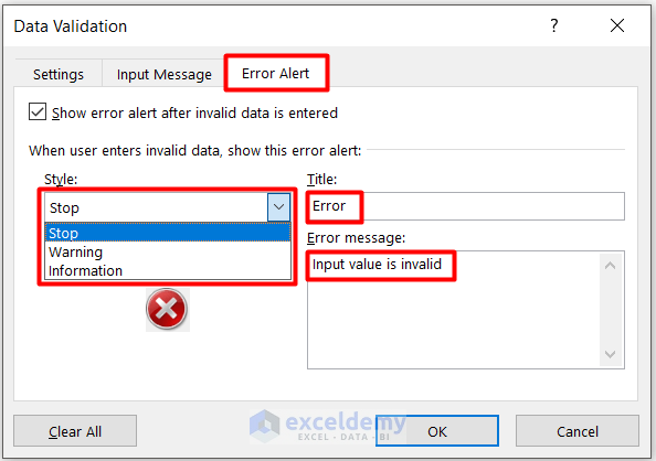
- To change the error message, click on the Error Alert tab.
- Change the Style, Title and Error message as desired.
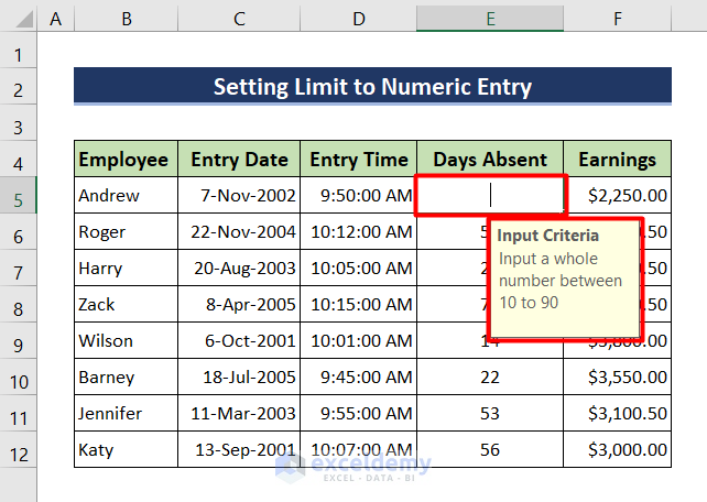
In the following figure, when you select cell E5, the Input Message will appear.
If you put an invalid value in the cell, it will show the Error Alert you created.
Read More: How to Use Excel Formula Not to Exceed a Certain Value
1.2 – Decimal Numbers Only
Steps:
- Select all the cells in which to set the limit to decimal numbers. Here, column F.
- Go to the Data Validation tool from the Data Tab.
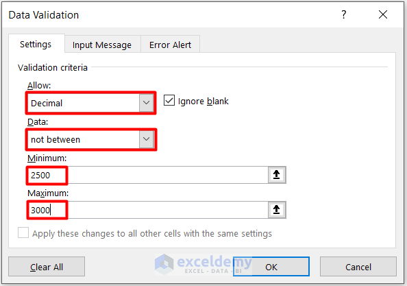
- In the pop-up box that opens, select Decimal in the Allow option and choose any suitable criteria in the Data menu.
Here, we chose not between, which only allows values which are not within the specified range, and a not between range of 2500-3000.
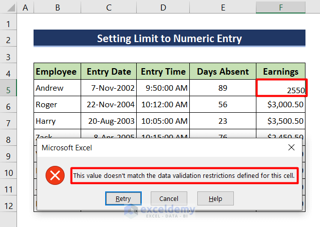
If we try to enter the value 2550, which is in the range, an error message will pop up.
Read More: How to Make a Data Validation List from Table in Excel
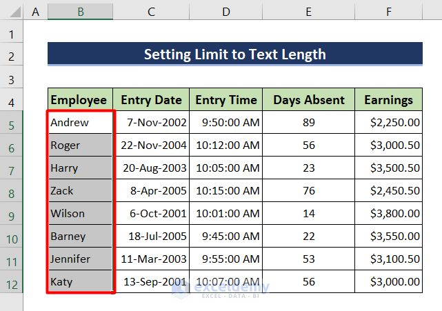
Method 2 – Set Limit to Text Length
Steps:
- Select all the cells of the Employee column. We will limit the text length to 10 in these cells.
- Go to the Data tab.
- Select Data Validation from the ribbon.
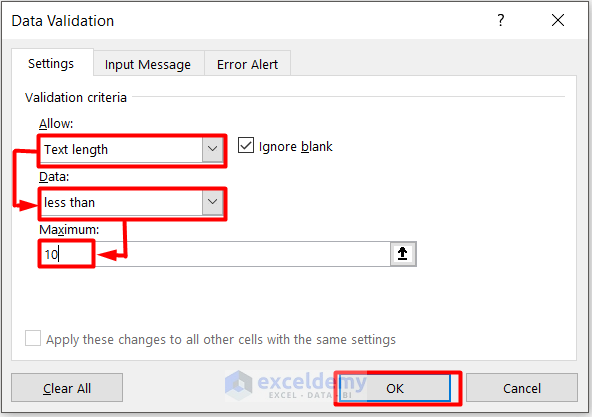
- In the pop-up box that opens, select Text length in the Allow option and choose any convenient criteria in the Data.
We selected the less than option and chose the maximum value as 10. This will allow text with less than 10 characters only.
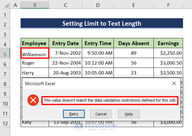
- To check if it works, enter any name containing more than 10 characters in the selected cells.
We wrote Williamson which has more than 10 characters. We receive an error message that the data doesn’t match the input criteria.
Method 3 – Limiting Cell Entry to a List
We will now limit cell entries to only the data in a list.
Steps:
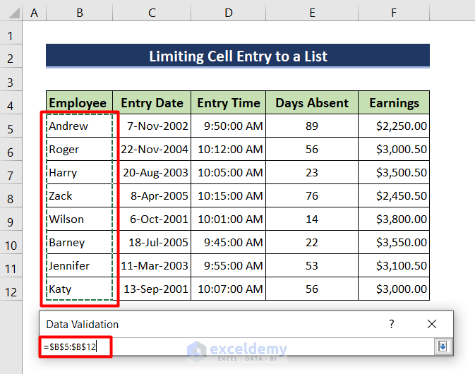
- Select cells B5 to B12.
- Go to the Data Validation tool from the Data Tab.
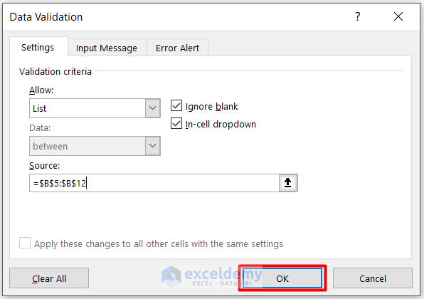
- In the Data Validation window, select List in Allow.
- Click on the arrow of the source cell.
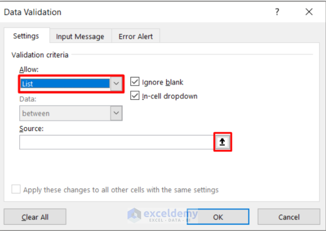
- Select the range of the list of allowed terms for entry. We specified the range from B5 to B12.
- Click OK.
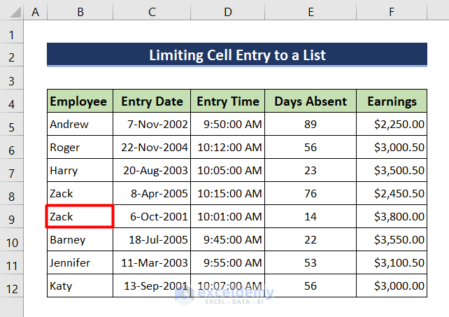
Now if we type any name in the specified list, the cell will accept it. Here, we wrote the name Zack in cell B9, which the cell accepted.
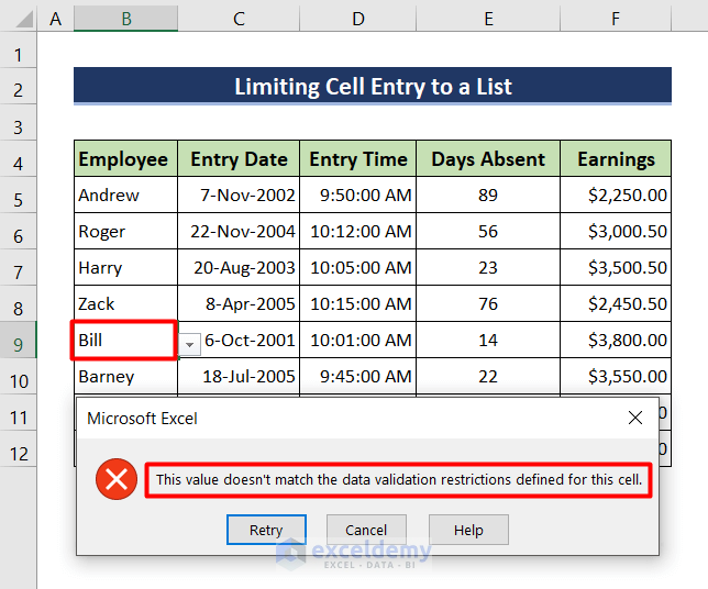
On the other hand, when we typed the name Bill which was not on the list, an error message popped up.
Read More: How to Use Data Validation List from Another Sheet
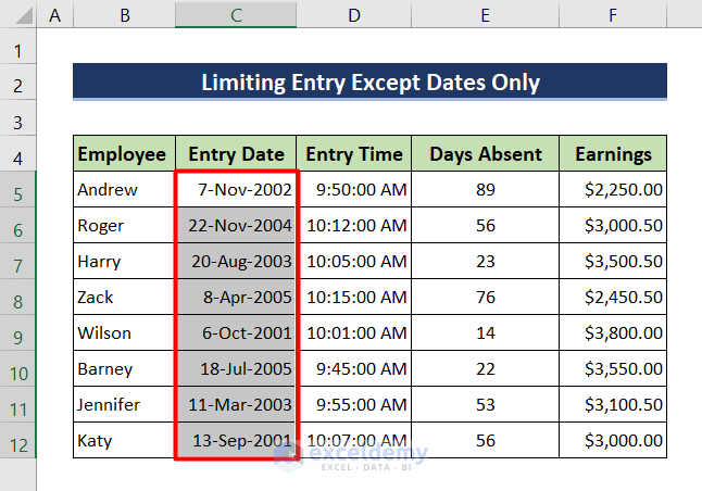
Method 4 – Limiting Entry to Date Values Only
Sometimes we need only dates in certain cells. We can do this by using the Data Validation tool.
Steps:
- Select the cells under Entry Date.
- Go to the Data Tab and click on the Data Validation tool.
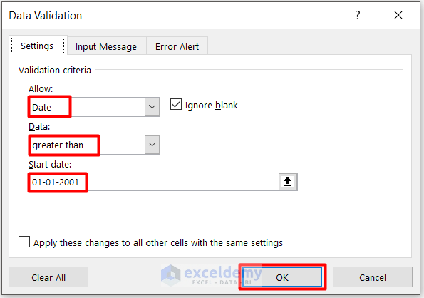
- Select Date in the Allow option.
- Choose any criteria in the Data option. We chose greater than and wrote the Start date as 01-01-2001, so any date before this date will be rejected.
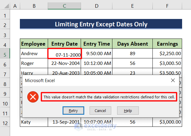
For instance, if we select C5 cell and type 07-11-2000 which does not meet the criteria, a pop-up will open and show an error.
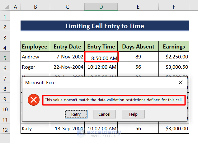
Method 5 – Limiting Cell Entry to Time
Now we will limit our cells to Time format.
Steps:
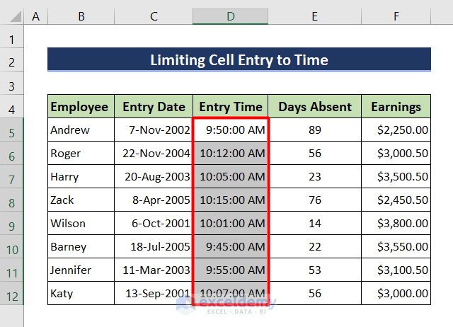
- Select the cells from D5 to D12.
- Click on the Data Validation tool from the Data Tab.
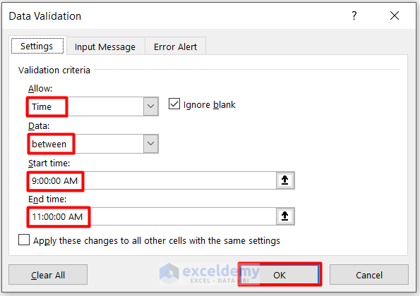
- In the Data Validation pop-up, select Time in the Allow option and choose any criteria according to your need. We selected the between criteria and chose the Start time and End time as 9:00:00 AM and 11:00:00 AM. This will allow times between 9 AM and 11 AM.
- Click OK.
- To see that it works, try to input a wrong value in cell D5.
We wrote 8:50:00 AM in the cell and an error message popped up.
Things to Remember
- Choose the limit criteria properly or you won’t get your desired results.
- Choose Custom in the Allow option of Data Validation if you need customized criteria.
Download Practice Workbook
Related Articles
<< Go Back to Data Validation in Excel | Learn Excel
Get FREE Advanced Excel Exercises with Solutions!
