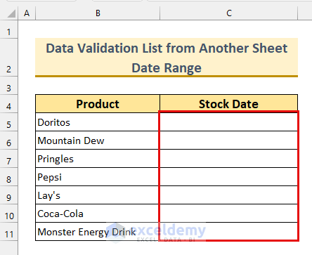
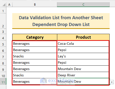
The below dataset has two columns: The Product purchased by a customer will be inserted using the Data Validation drop-down list from another sheet.
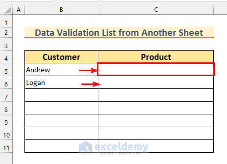
Method1 – Using a Data Validation List to Create a Drop-Down List from Another Excel Sheet
Steps:
- Select cell range B5:B11 from the “dropdown” sheet.
- From Data tab >>> Data Validation.
The Data Validation dialog box will appear.
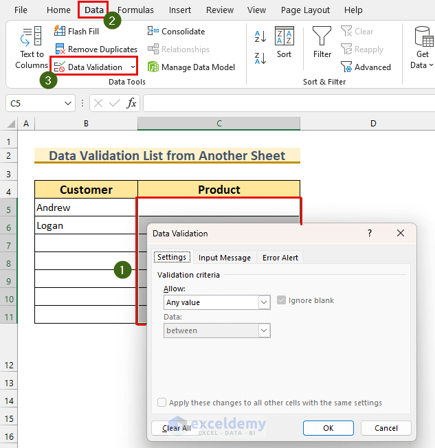
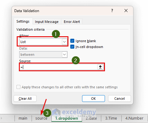
- Select List from the Allow drop-down menu.
Note: Ignore blank and In-cell dropdown should be checked by default. If not, put a tick mark beside those.
- Click on the Source box.
- Select the “source” sheet.
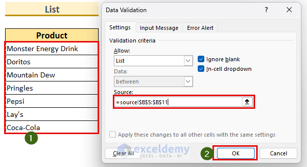
- Select the cell range B5:B11. This is our validation list.
- Press OK.
- Click on the arrow icon.
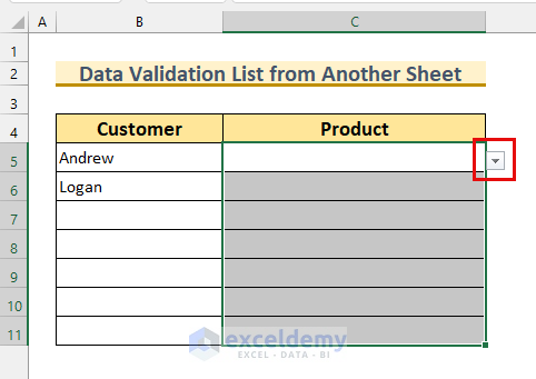
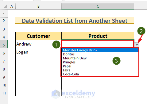
We can see our Data Validation list from another sheet.
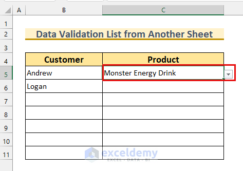
- Choose anything from the list.
The value will be inserted into our dataset.
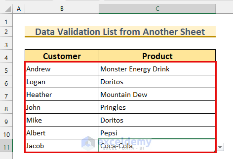
Here, we’ve filled our dataset using the Data Validation list from the other sheet in Excel.
Read More: How to Make a Data Validation List from Table in Excel
Method 2 – Applying Date Range by Using Data Validation List From Another Sheet
The dataset has an empty stock date column for the products. We’ll populate this using the Data Validation list. This time, we’ll use the Date between option.
Steps:
- Select cell range C5:C11.
- Bring up the Data Validation dialog box.
- Choose these settings:
- Allow: Date.
- Data: between.
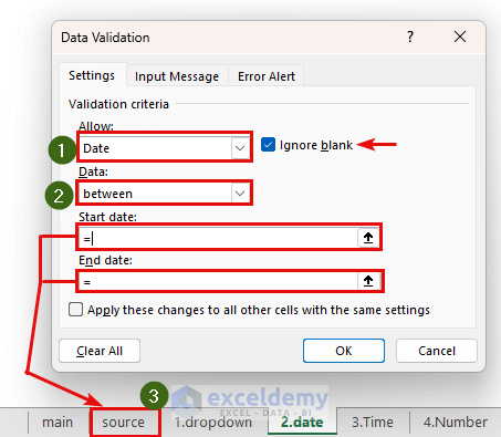
- Choose the cell reference from the “source” sheet.
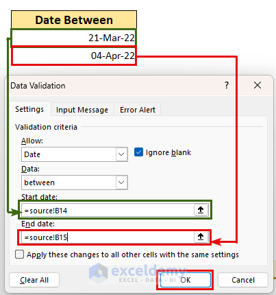
- Start date: B14 cell from “source” sheet.
- End date: B15 cell from “source” sheet.
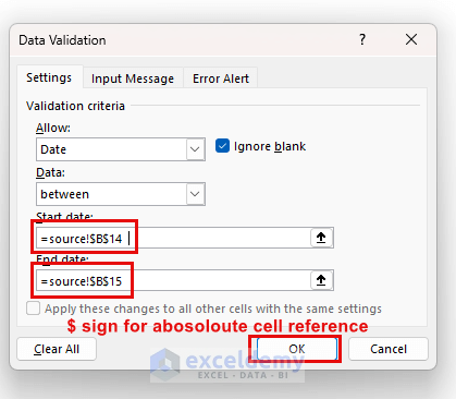
Sometimes, we need to use an absolute cell reference in our data. This will ensure that our data doesn’t change when we move to another cell.
- Press OK.
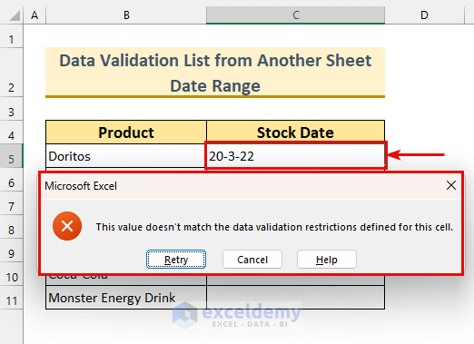
If we enter anything other than our defined criteria, then we’ll get an error message. This message can be modified.
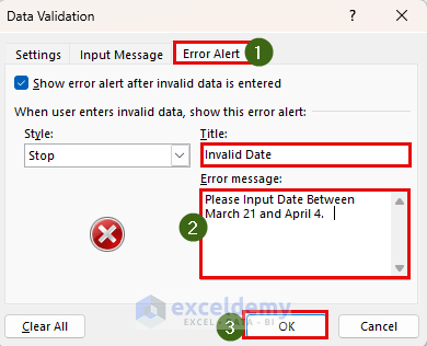
We can change the message by going to the Error Alert tab from the Data Validation dialog box.
- Enter something in the Title: This is an optional task.
- Customize the message by typing in the Error message:
- Press OK.
We see our custom error message is working.
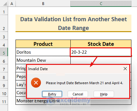
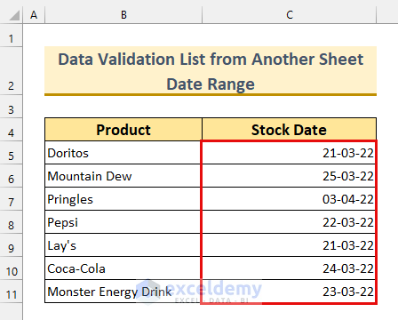
We can manually type the dates into the rest of the fields. A warning message will be shown if we type something beyond the date range. That is how we can apply the Data Validation list to restrict our cells.
Method 3 – Fixing Time Limit by Applying Data Validation List from Another Excel Sheet
The Data Validation list to limit our time input in the cells. That list is on another sheet. We will input time within our criteria in the Stock Time column.
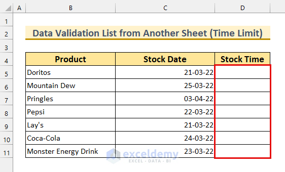
Steps:
- Select the cell range D5:D11.
- bring up the Data Validation dialog box.
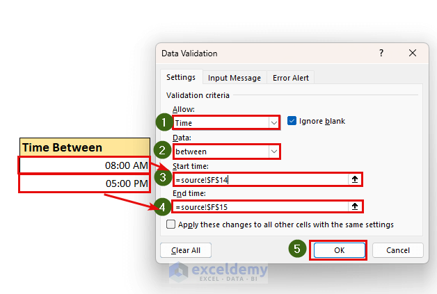
- Choose these options:
- Allow: Time.
- Data: between.
- Start time: cell F14 from the “source” sheet.
- End time: cell F15 from the “source” sheet.
- Press OK.
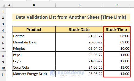
We can populate the Stock Time column between 8 AM and 5 PM.
Method 4 – Getting Greater Numbers with Excel Data Validation List From Another Sheet
Another column has been added to our dataset. We’ll use the greater than criteria for the whole number to apply the Data Validation list.
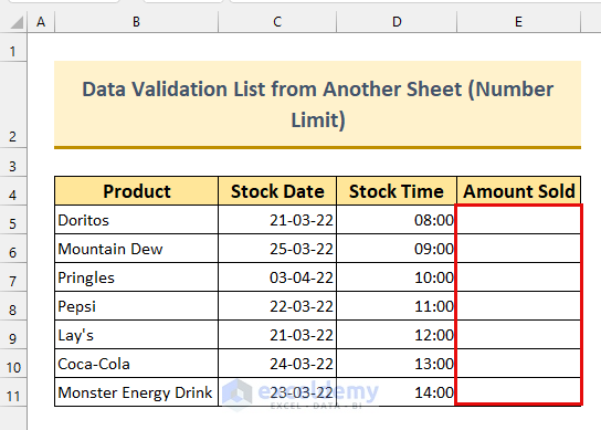
Steps:
- Select cell range E5:E11.
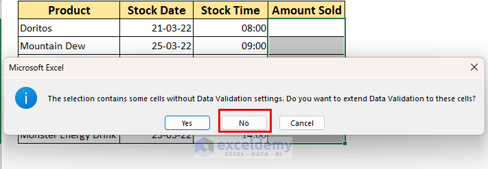
- From the Data tab, bring up the Data Validation dialog box.
You may get a similar warning message. Click NO.
- From the dialog box, choose these:
- Allow: Whole number.
- Data: greater than.
- Minimum: cell F7 from the “source” sheet.
- Press OK.
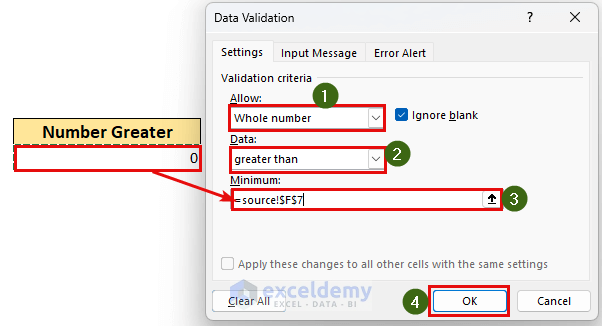
We can put values greater than 0 in the Amount Sold column. This Data Validation list can help us avoid typing wrong values.

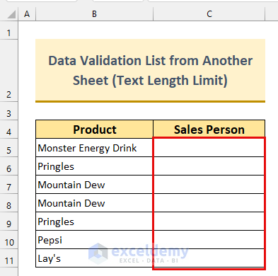
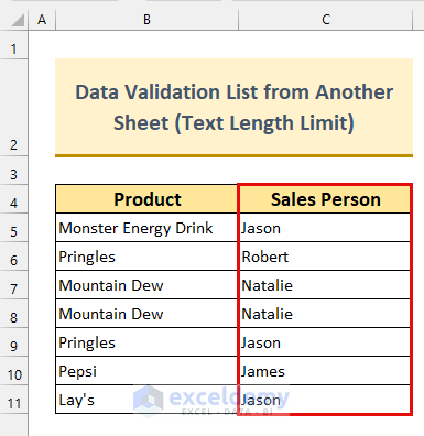
Method 5 – Applying Data Validation List from Another Sheet to Limit Text Length
Below is a new dataset. We’ll input the Salesperson associated with a Product sale. We’ll only input short names.
Steps:
- Select cell range C5:C11.
- bring up the Data Validation dialog box from the Data tab.
- Choose these options:
- Allow: Text length.
- Data: between.
- Minimum: cell B40 from “source” sheet.
- Maximum: cell B41 from “source” sheet.
- Press OK.
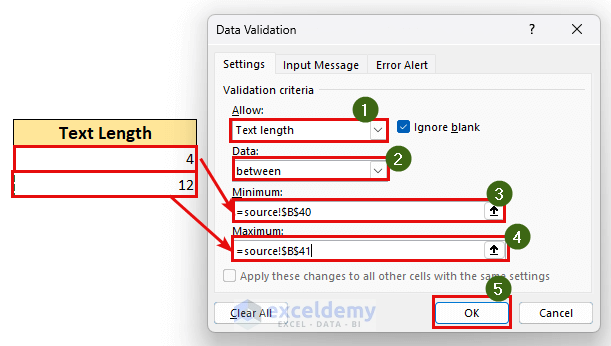
We can use our Data Validation list to fill the rest of the cells.
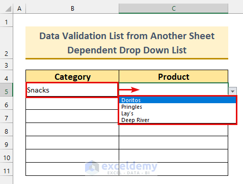
Method 6 – Using Data Validation List from Another Sheet to Create Dependent a Drop-Down List
We’ll create a dependent drop-down menu using the Data Validation list.
Steps:
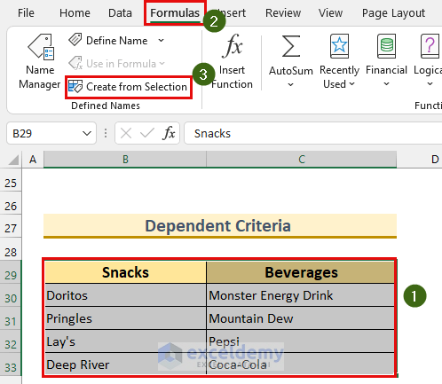
- Create a Named Range.
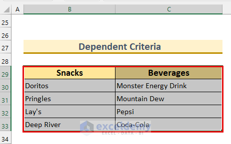
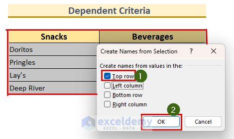
- Select the cell range B29:C33.
- From Formulas tab >>> Create from Selection.
A dialog box will appear.
- Select Top row.
- Press OK.
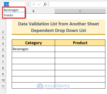
There is a Name Box at the top right corner. Click it to see our Named Range.
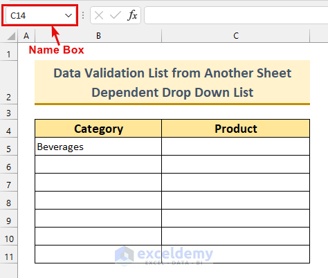
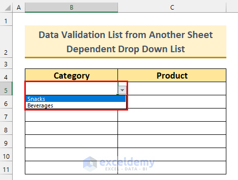
We see our two Named Ranges: Beverages and Snacks.
- Select cell B4.
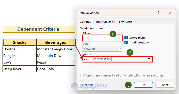
- Bring up the Data Validation dialog box from the Data tab.
- Choose these settings:
- Allow: List.
- Source: select cell range B29:C29.
- Press OK.
The B5 cell shows the two categories.
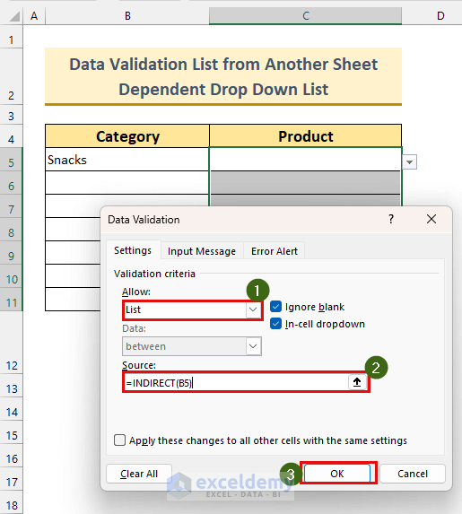
- make a dependent list in cell C5.
- Select the cell range C5:C11.
- From the Data tab, bring up the Data Validation dialog box.
- Set these values:
- Allow: List.
- Source: Type the following formula there.
=INDIRECT(B5)- Press OK.
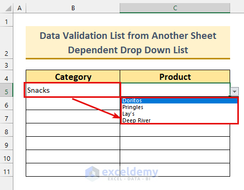
In cell C5, products from the Snacks category are shown.
If we change cell B5 to Beverages, then cell C5 will change.
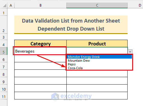
We can do this for the rest of the cells and fill them with dependent values.
Read More: Excel Data Validation Drop Down List with Filter
Download the Practice Workbook
Related Articles
<< Go Back to Data Validation in Excel | Learn Excel
Get FREE Advanced Excel Exercises with Solutions!
