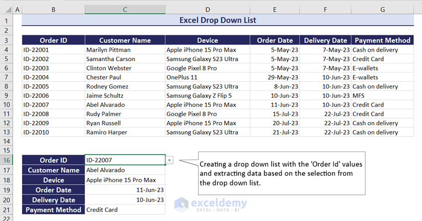
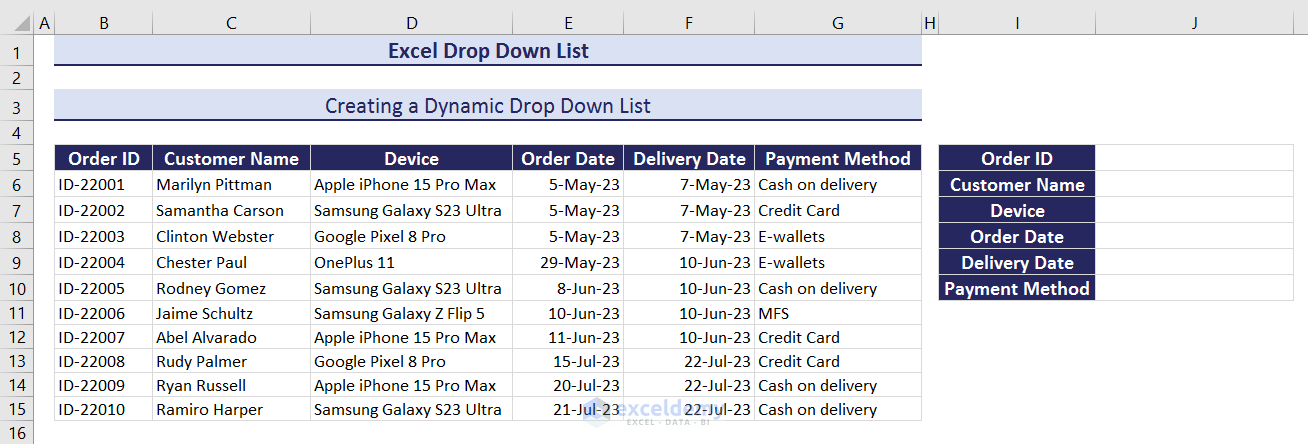
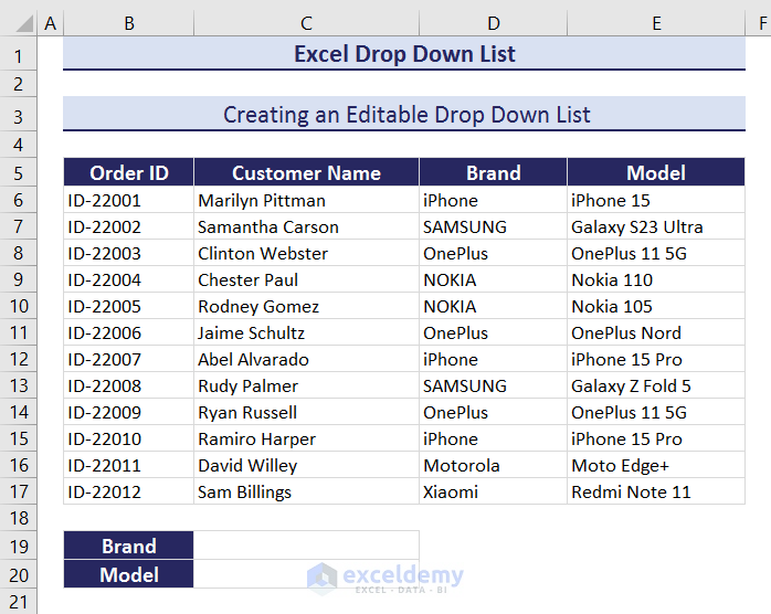
The dataset showcases online shopping information: ‘Order ID’, ‘Customer Name’, ‘Device’, ‘Order Date’, ‘Delivery date’, and ‘Payment Method’.
What Is a drop-down List in Excel?
A drop-down list is a feature that allows users to select an element from a list of options.
How to Create a drop-down List in Excel?
1. Creating a drop-down List from a Cell Range
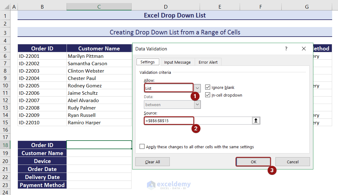
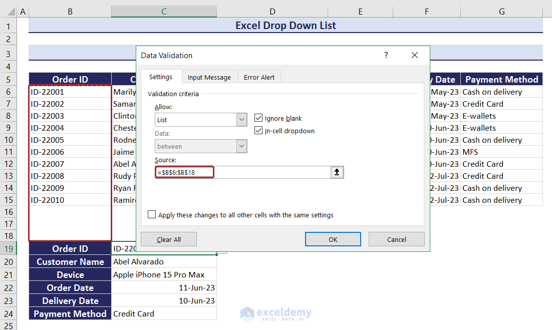
To create a drop-down list based on the values in column B:
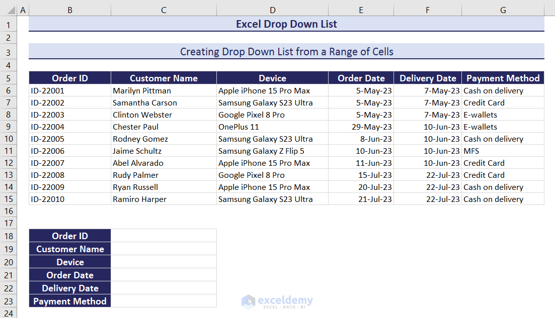
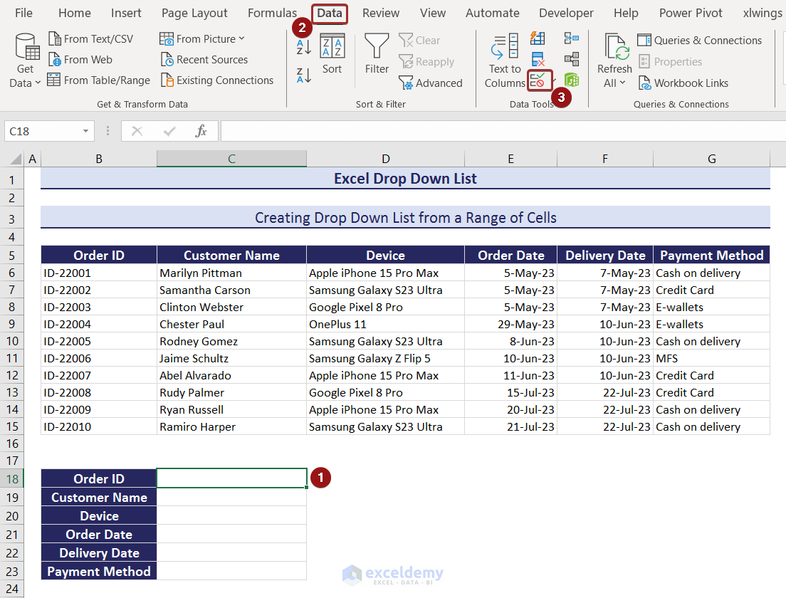
- Select a cell (C18).
- Go to the Data tab and select Data Validation.
- In Data Validation, go to Setting.
- In List, choose Allow.
- Define a range ($B$6:$B$15) in Source.
- Click OK.
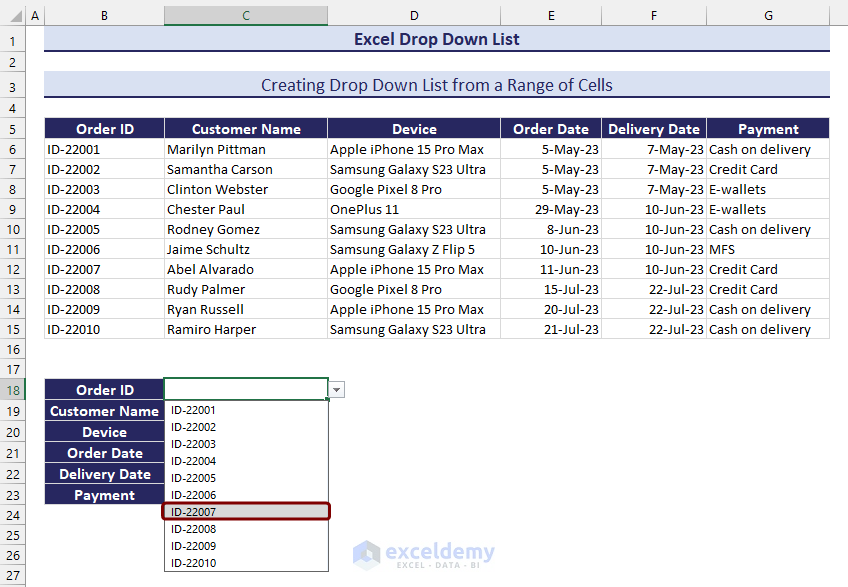
This is the output.
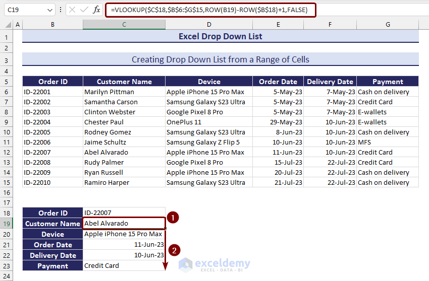
- Enter the following formula in C19 to have the value from column C, based on the Order ID selection.
=VLOOKUP($C$18,$B$6:$G$15,ROW(B19)-ROW($B$18)+1,FALSE)- Use the Fill Handle to extract values.
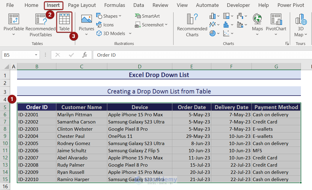
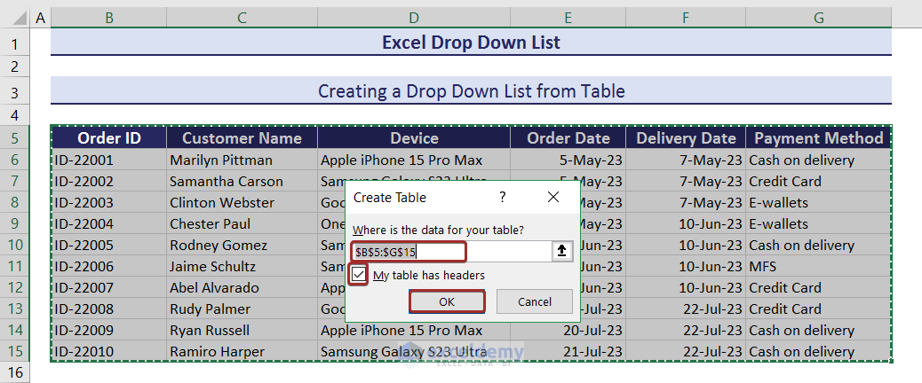
2. Creating a drop-down List from a Table
- Select a cell range and go to the Insert tab to create a table.
- Click Table.
- Check My table has headers.
- Click OK.
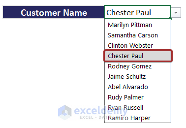
- To create a drop-down list in C18 with data in Customer Name, select List in Allow.
- Enter the following formula with the INDIRECT function in the Source and click OK.
=INDIRECT("Table1[Customer Name]")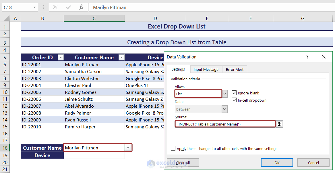
- Enter the following formula in C19 to extract the device name based on the customer name selection.
=INDEX(Table1,MATCH(C18,Table1[Customer Name],0),3)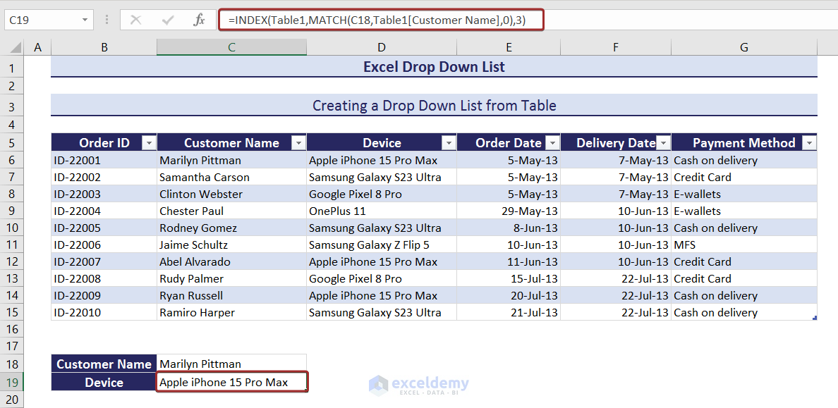
This is the output.
3. Creating a drop-down List with a Named Range
- Select a cell range and go to the Formulas tab.
- Click Define Name.
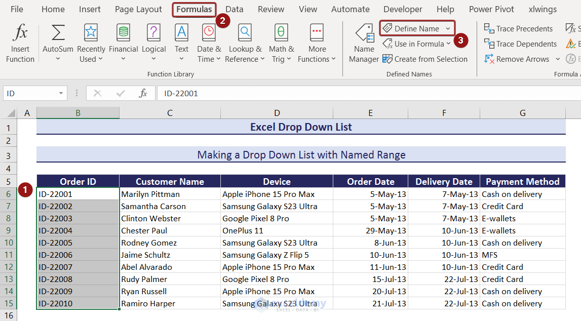
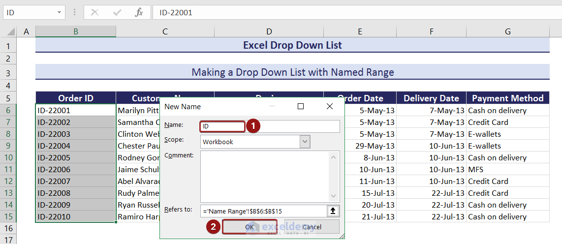
- Set a name (ID) in Name and define a range in Refers to.
- Create a drop-down list of order IDs in C19 by entering the following formula in Source:
=ID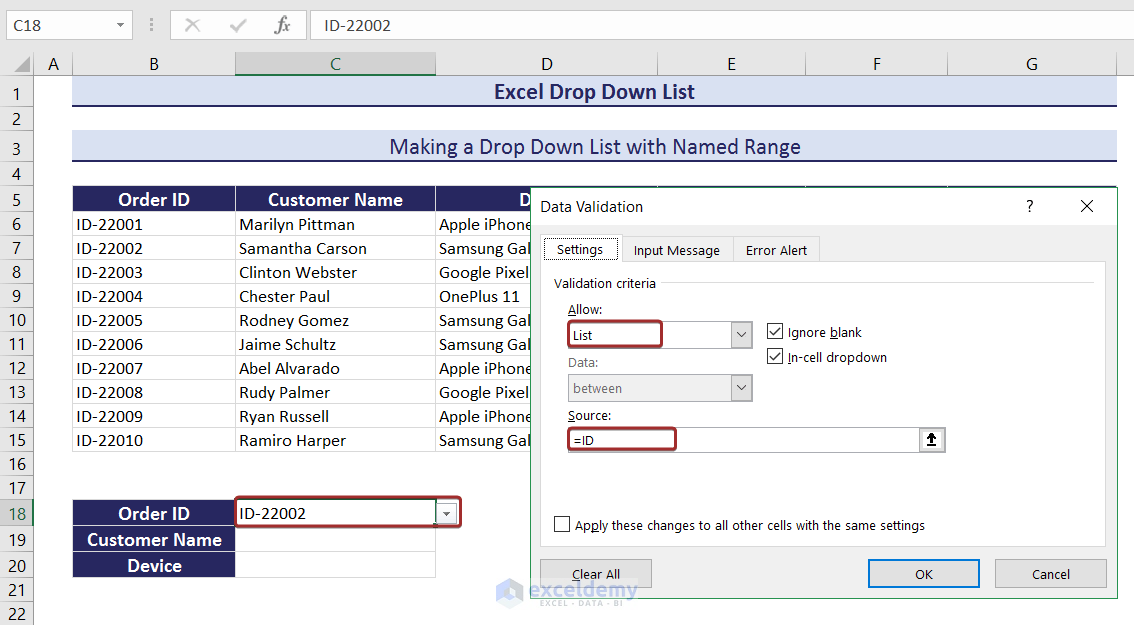
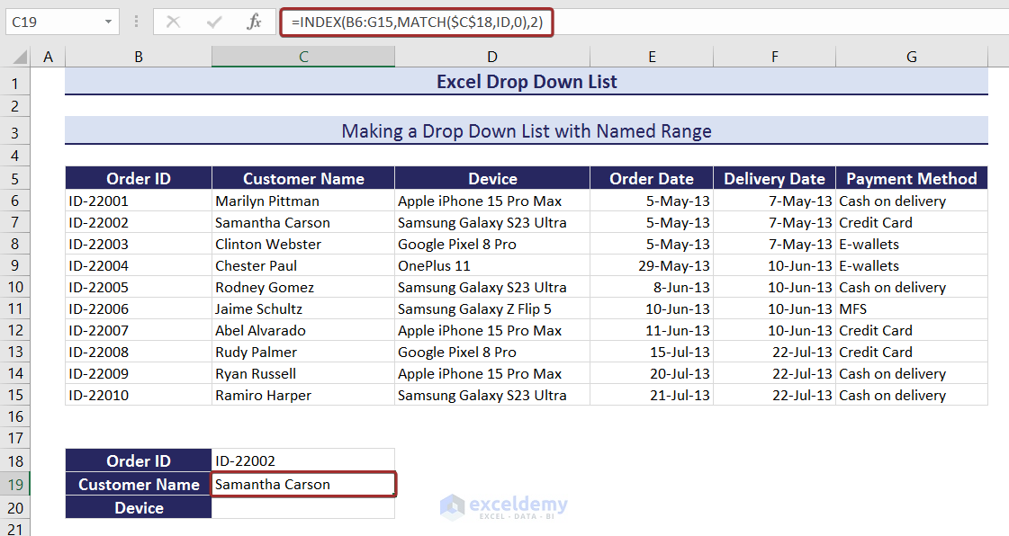
- Use the following formula in C19 to have the customer name based on the order ID selection.
=INDEX(B6:G15,MATCH($C$18,ID,0),2)
- Use the following formula to have the name of the device in C20.
=INDEX(B6:G15,MATCH($C$18,ID,0),3)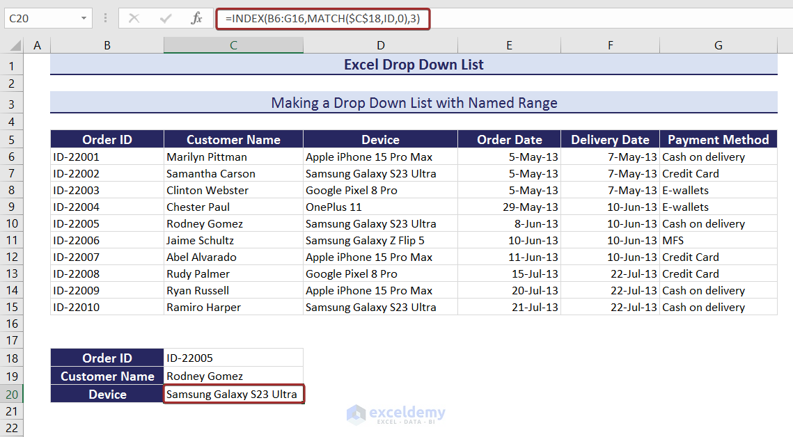
This is the output.
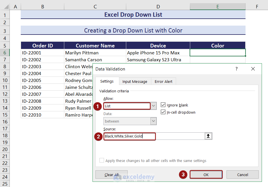
4. Creating a drop-down List with Color
Define a custom color with Conditional Formatting for each value of the drop-down list.
- Select List in Allow .
- Enter the color names separated by a comma sign (,): ( Black,White,Silver,Gold) in Source.
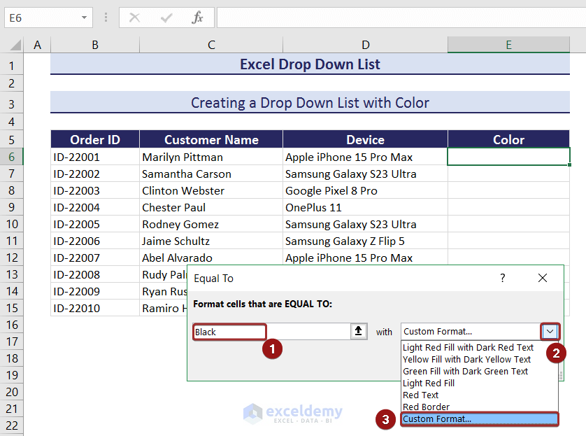
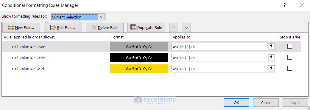
- To define a color for each of the elements of the drop-down, select the drop-down and go to Conditional Formatting in the Home tab.
- Go to Highlight Cell Rules and click Equal To…
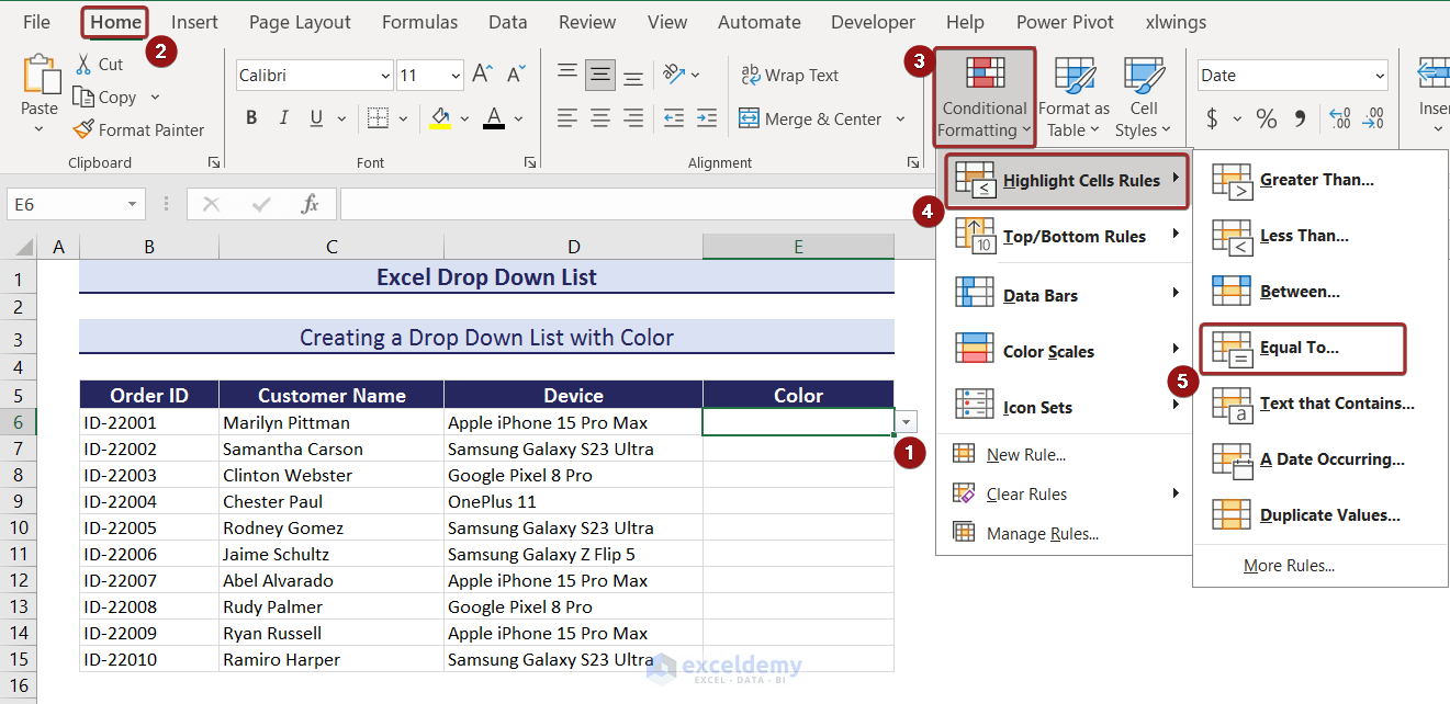
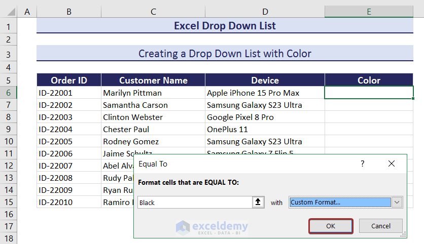
- In Equal To, enter the name of the color (Black).
- Select Custom Format to set a color for the color name.
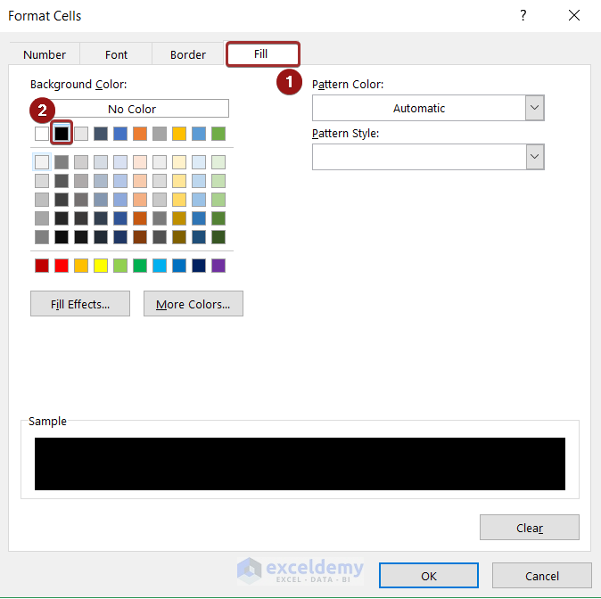
- Choose a color in Fill.
- You can also change the font color in Font. Here, white.
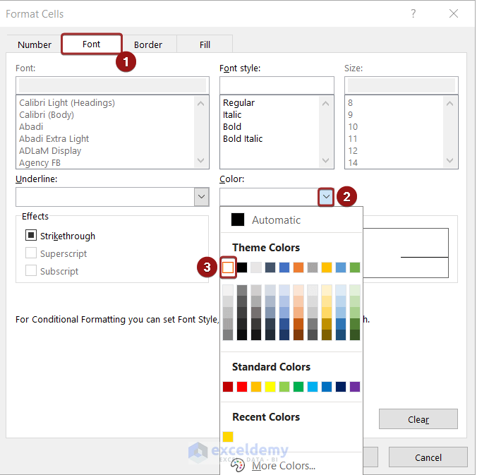
- Click OK.
- Set colors for the other options.
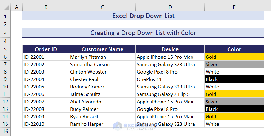
The drop-down list displays color based on the cell value.
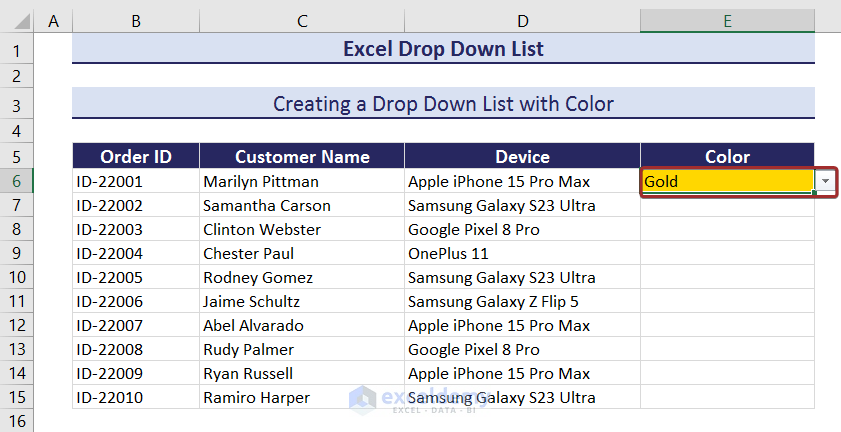
Color will automatically change based on the selection.
- Use the Fill Handle to AutoFill the drop-down.
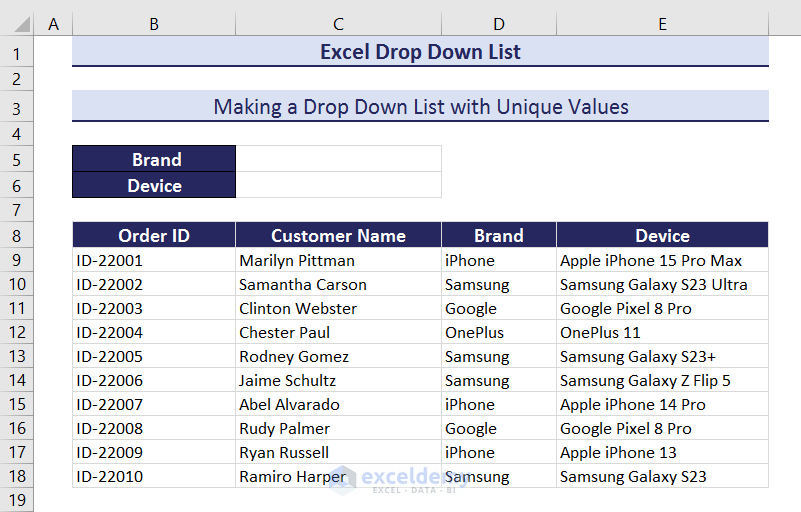
5. Creating a drop-down List with Unique Values
Create drop-down lists with the unique values in columns D and E.
- Use the following formula in B22 to see the unique brand names.
=UNIQUE(D9:D18)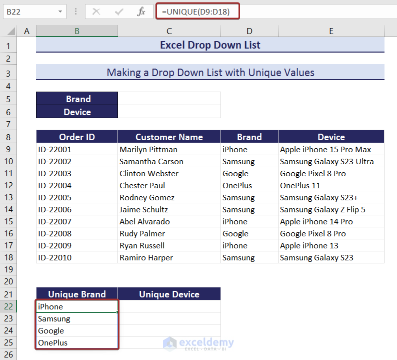
- Enter the following formula to create a drop-down list in C5 with unique values.
=$B$22:$B$25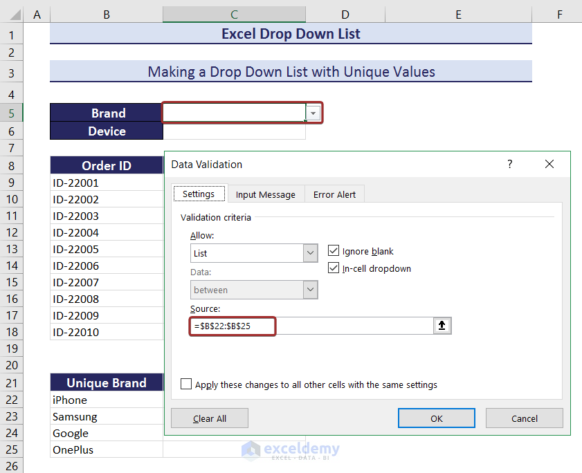
- Enter the following formula in C22 to see the unique values in column E that match the brand in C5.
=FILTER(E9:E18,C5=D9:D18)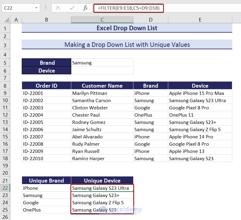
- Go to Data Validation.
- Use the following formula in Source.
=$C$22$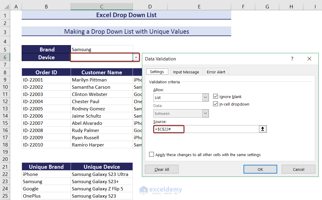
This is the output.
6. Creating a drop-down List Based on Data from Another Sheet
Mobile brands and their phone models are in the PhoneList worksheet.
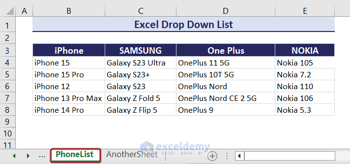
Use the brand names and phone models to create two drop-down lists in another worksheet (AnotherSheet).
- To create a drop-down list of brand names in D6 with the data in the PhoneList worksheet, enter the following formula in Source.
=PhoneList!$B$3:$E$3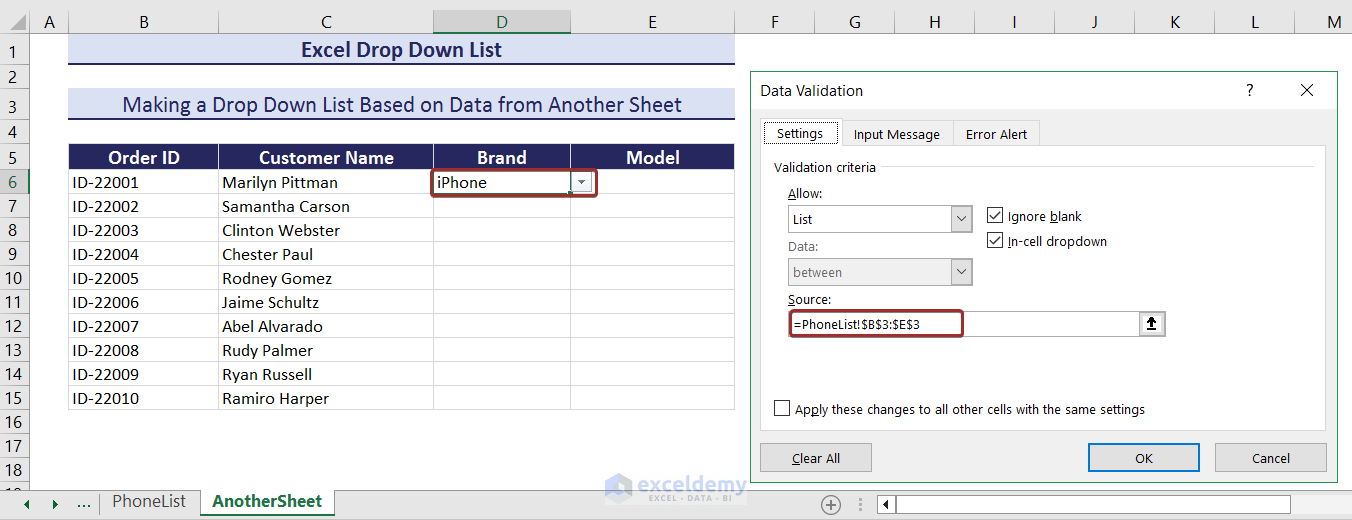
- Use the Fill Handle to create the same drop-down list in column D.
- Use the following formula with the INDIRECT function in Source to have the phone models from the PhoneList worksheet in a drop-down based on the brand names in column D.
=INDIRECT($D6)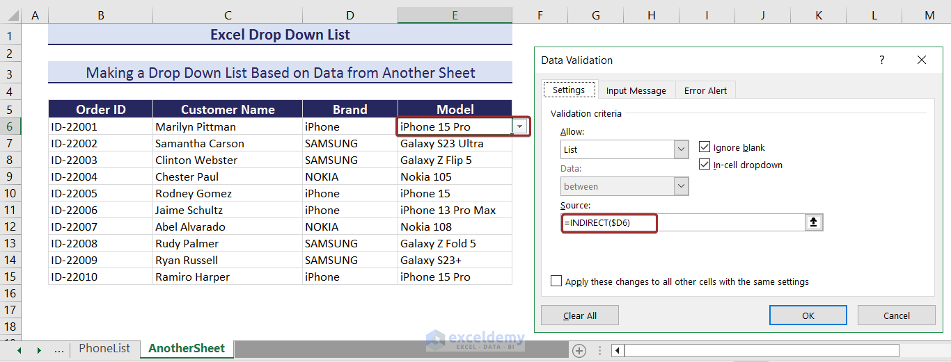
Click here to enlarge the image.
This is the output.
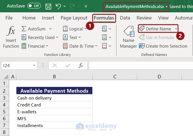
7. Creating a drop-down List Based on Data from Another Workbook
In the AvailablePaymentMethods workbook, there is a list of payment methods for online shopping.
- Go to Formulas and select Define Name.
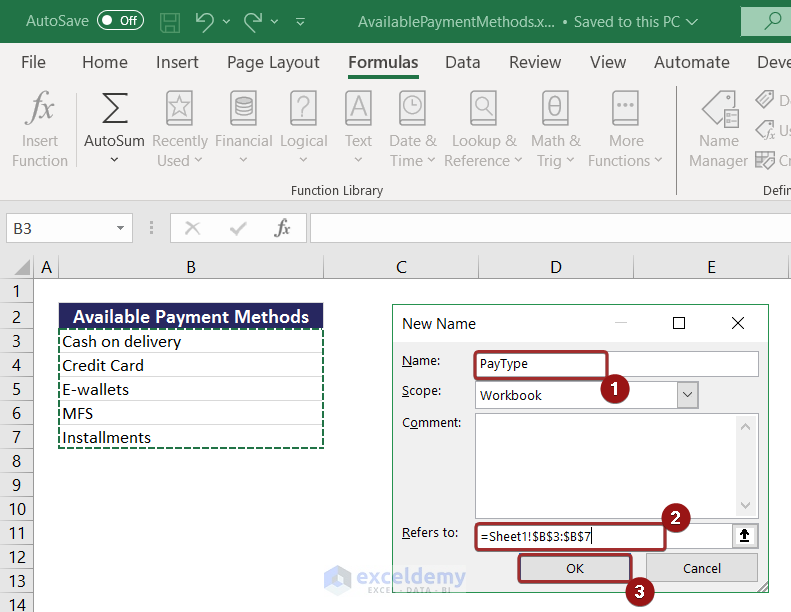
- In New Name, define a name (PayType) in Name.
- Define a range (Sheet1!$B$3:$B$7) in Refers to.
- Click OK.
- Go to the drop-down in Excel workbook and set a named range (PayType).
- Enter [AvailablePaymentMethods.xlsx]Sheet1!PayType to define the name range in the AvailablePaymentMethods workbook.
- Enter the following formula in Source to create a drop-down list with the named range in G6.
=PayType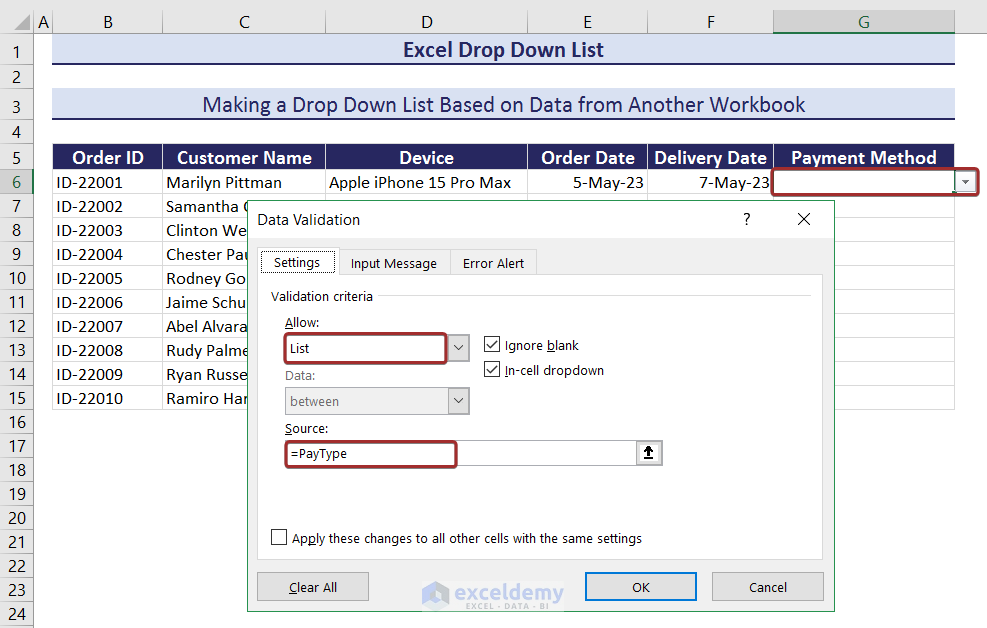
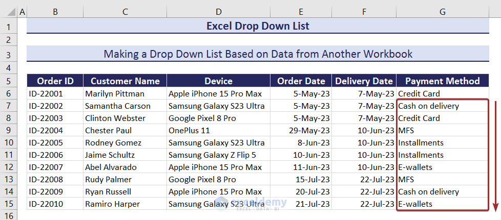
- You can select a payment method from the drop-down list.
- Use the Fill Handle to AutoFill the drop-down list.
ii. Don’t create multiple dependent drop-down lists from another workbook.
8. Creating a Dependent drop-down List
- To create an independent drop-down list of brands in D6, enter the following formula in Source (Data Validation).
=$B$18:$E$18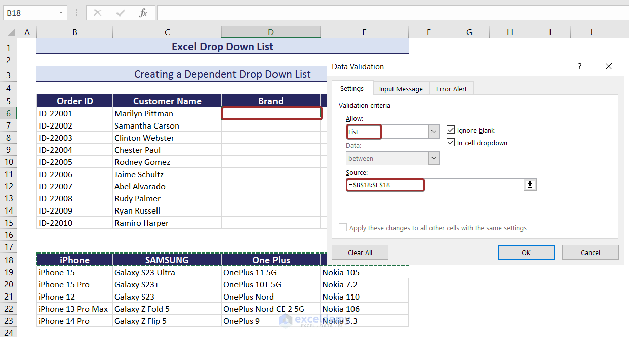
- To create the dependent drop-down list of phone models in E6, enter the following formula with the INDIRECT function in Source.
=INDIRECT($D6)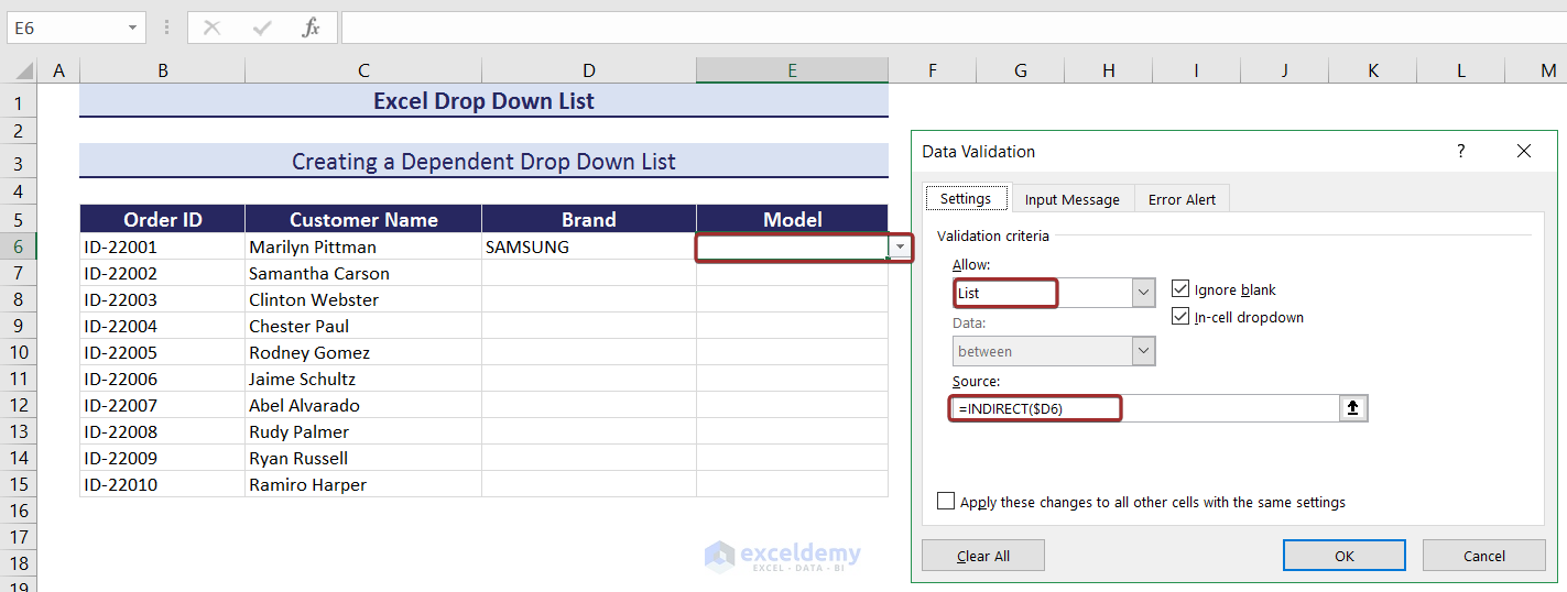
Click here to enlarge the image.
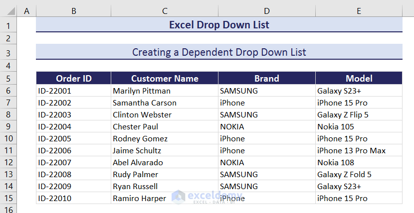
The dependent drop-down list based on the selection of brand from an independent drop-down list is created.
- Use the Fill Handle to AutoFill the drop-down lists.
9. Creating a Searchable drop-down List
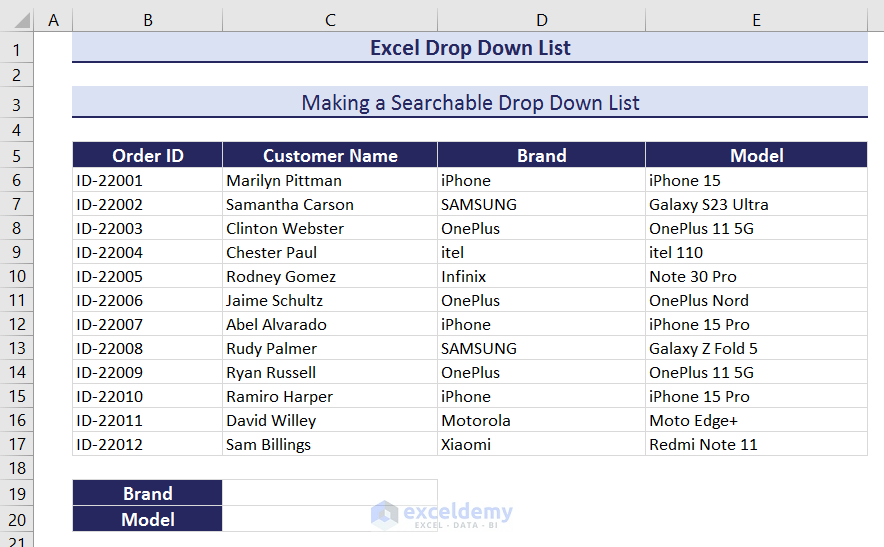
- Insert new columns (G and H) to have unique brand and model names. Use the following formula in G6.
=UNIQUE(OFFSET(D6,0,0,COUNTA(D:D)-1,1))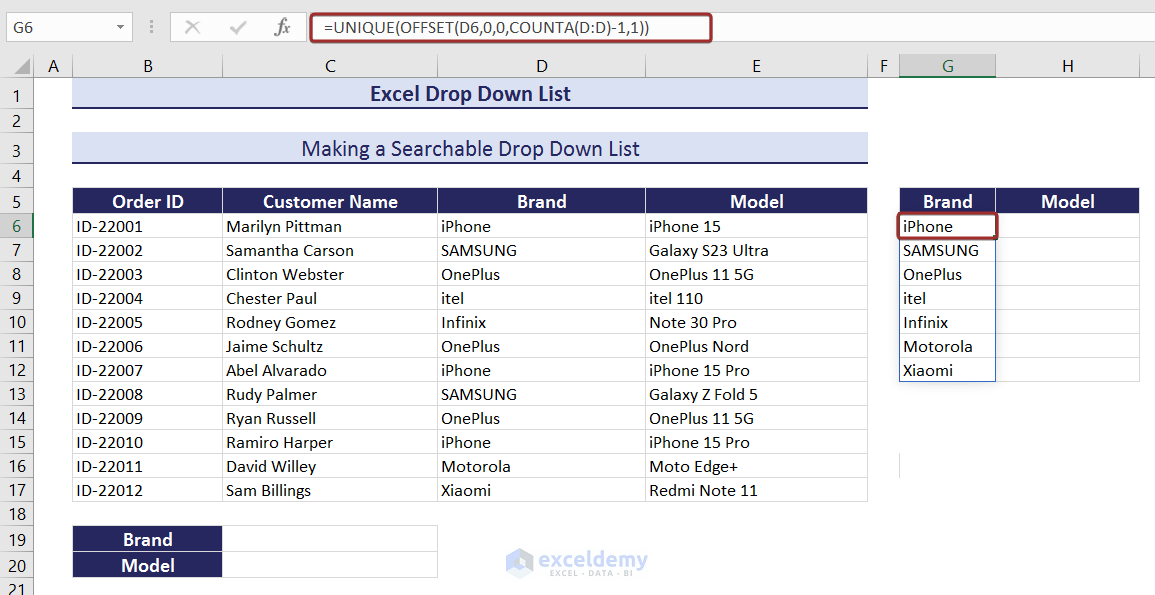
- Enter the following formula in Source to create a searchable drop-down list in C19 with the brand names.
=$G$6#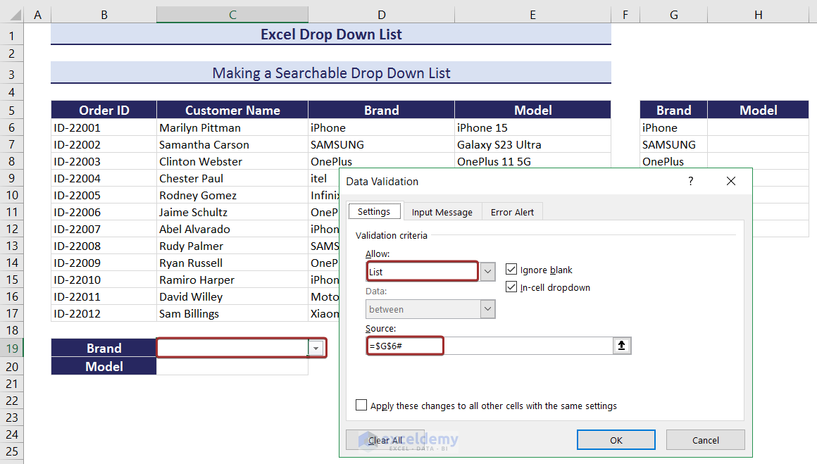
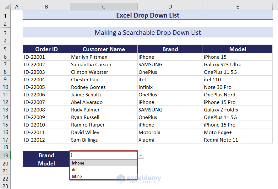
You will be able to search brand names in C19.
- Enter the following formula in H6 to see phone models based on the brand selection of the searchable drop-down.
=UNIQUE(FILTER(E6:E17,C19=D6:D17))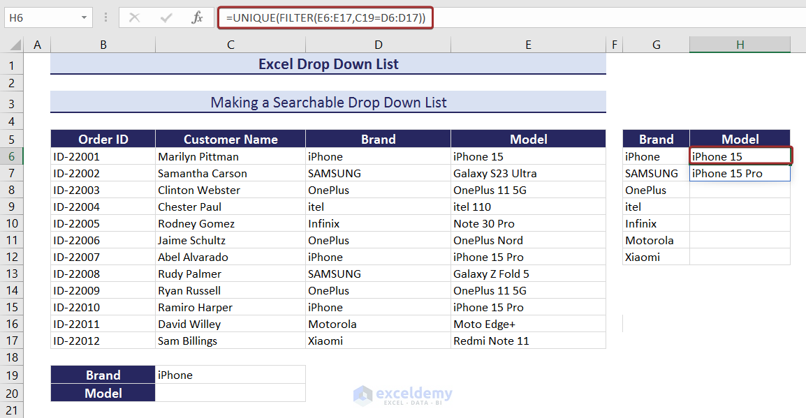
- Enter the following formula in Source to create a searchable drop-down in C20 with the phone model names.
=$H$6#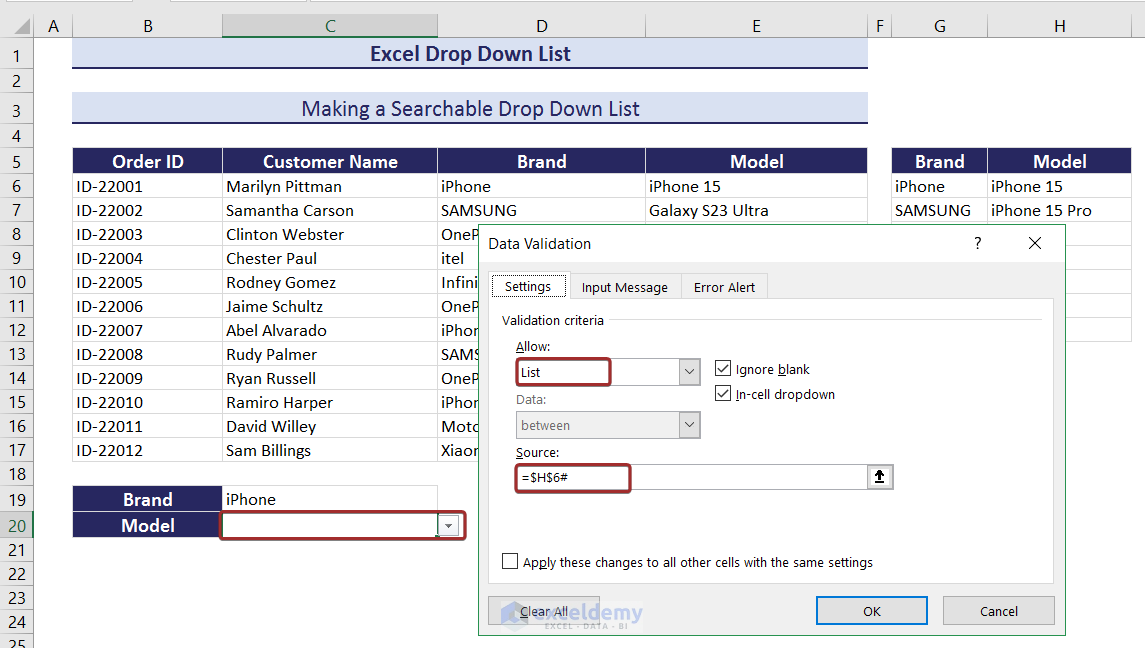
You have independent and dependent searchable drop-down lists.
10. Creating a Dynamic drop-down List to Add and Auto Update New Entries
To extract values based on the ID.
Click here to enlarge the image.
- Insert a separate column and enter the following formula in L6 to see unique IDs based on column B values.
=UNIQUE(OFFSET(B6,0,0,COUNTA(B:B)-3,1))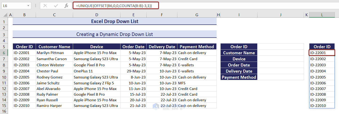
Click here to enlarge the image.
- Create a drop-down list with the unique IDs in J5 by entering the following formula in Source.
=$L$6#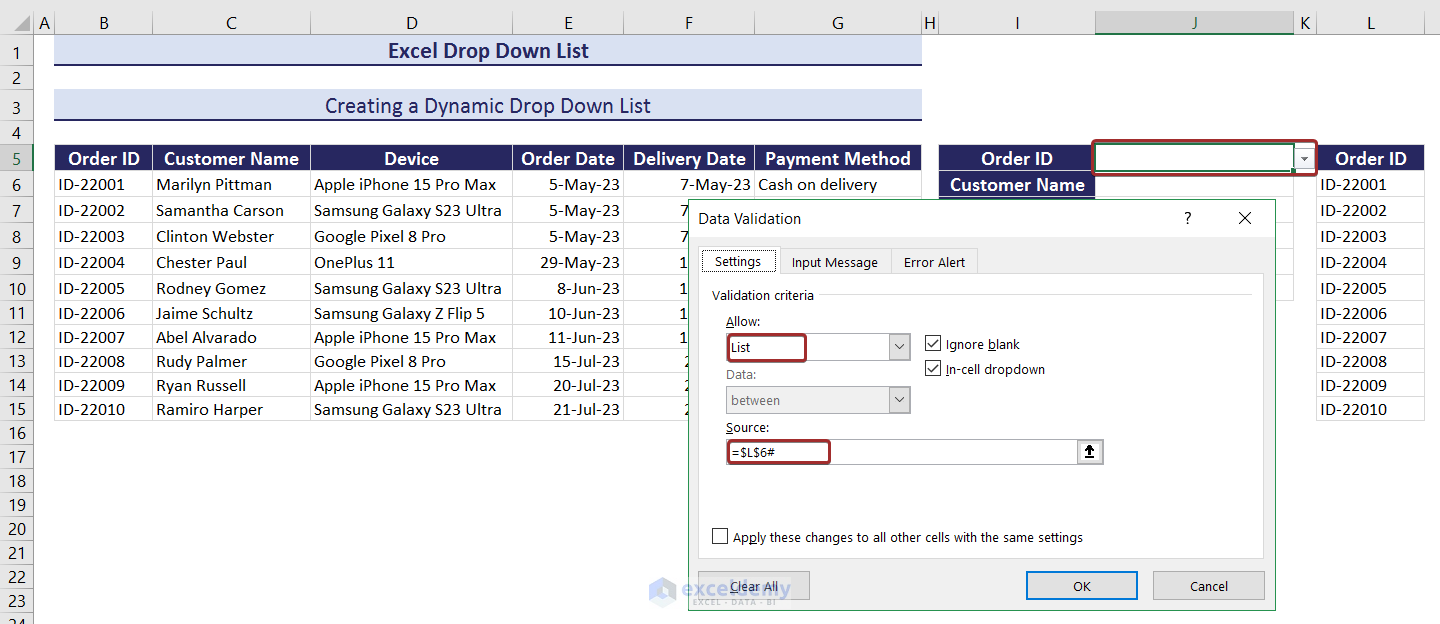
Click here to enlarge the image.
- Select an ID from the drop-down list and use the following formula in J6 to see the customer name for the selected ID.
=VLOOKUP($J$5,B:G,ROW(I6)-ROW($I$5)+1,FALSE)- Use the Fill Handle to AutoFill the rest of the values.
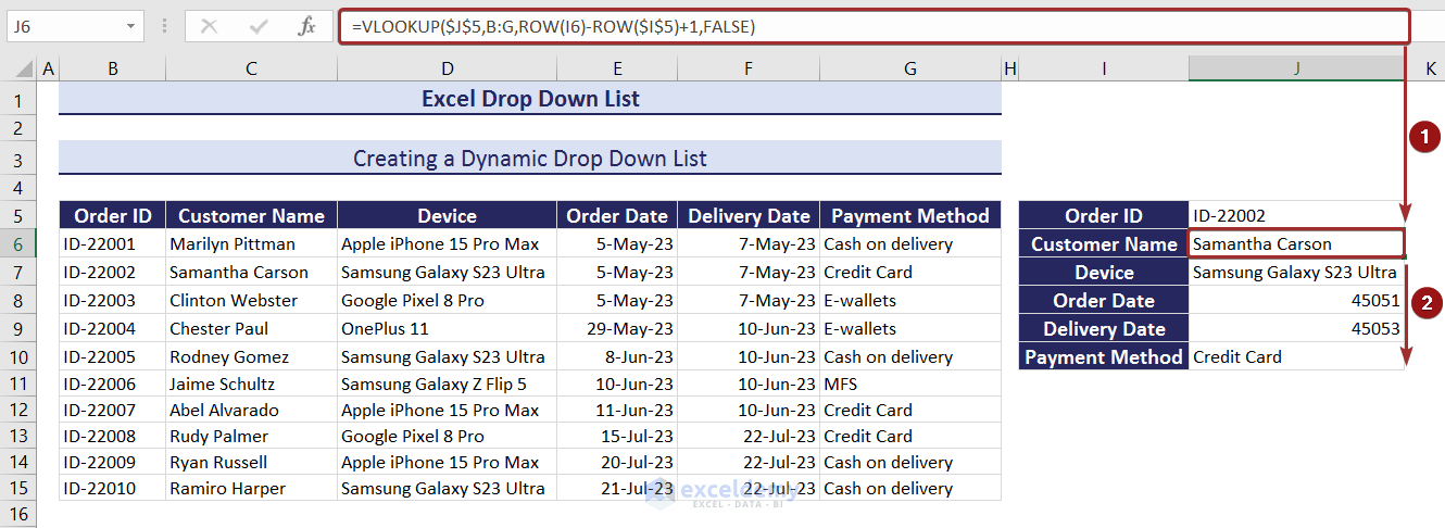
Click here to enlarge the image.
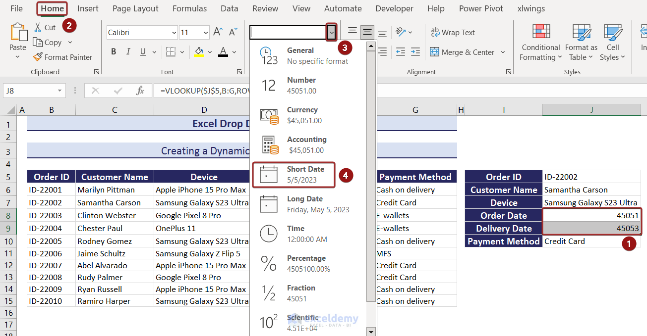
- The extracted dates will be shown as integer numbers. Change the number format to Short Date or Long Date in Number Format.
- Add extra IDs and their related values. They will automatically be updated in the drop-down list and in column L.
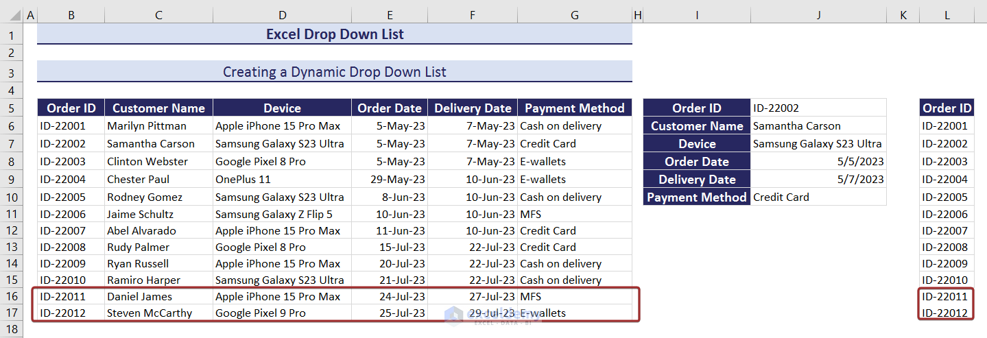
Click here to enlarge the image.
This is the output.
11. Creating a Searchable, Dynamic, and Multi-dependent drop-down List
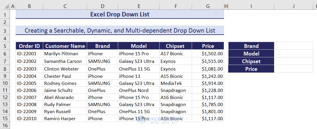
- Enter the following formula in L6.
=UNIQUE(OFFSET(D6,0,0,COUNTA(D:D)-1,1))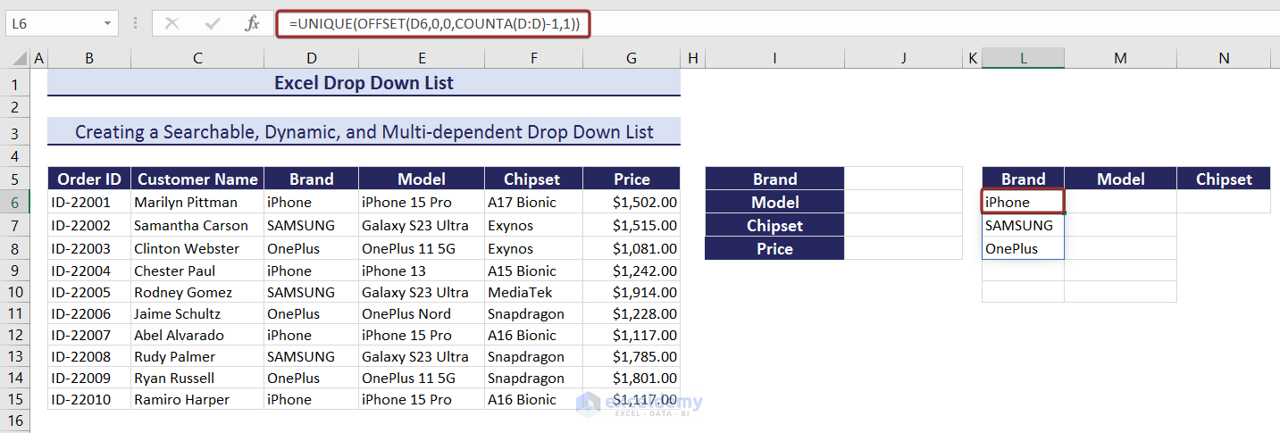
- Create an independent searchable drop-down list of brand names in J5 by entering the following formula in Source.
=$L$6#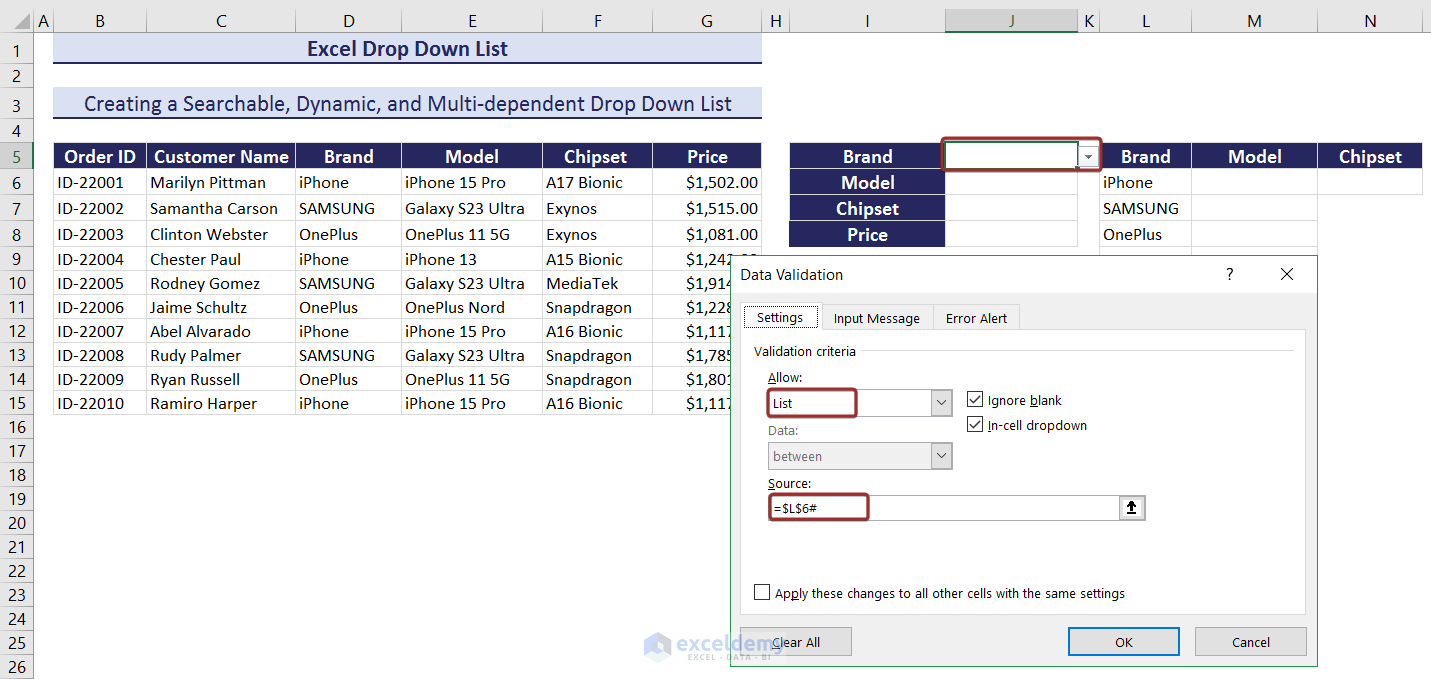
- Filter the phone models based on the brand selected from the drop-down list in J5. Use the following formula.
=UNIQUE(FILTER(E:E,J5=D:D))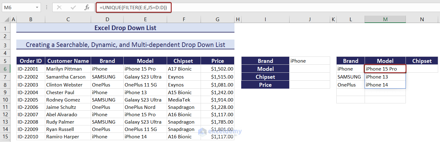
- Create a brand name dependent searchable drop-down list of phone model names in J6. Enter the following formula in Source.
=$M$6#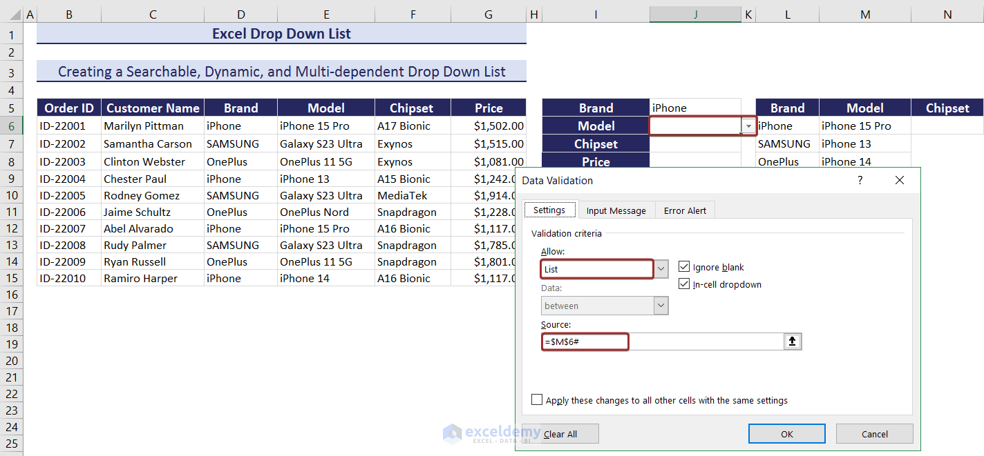
- Filter the chipsets based on the model selected from the drop-down list in J6. Use the following formula.
=UNIQUE(FILTER(F:F,J6=E:E))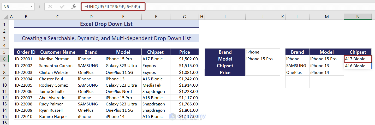
- Enter the following formula in Source to create a model name dependent searchable drop-down list of chipsets in J7.
=$N$6#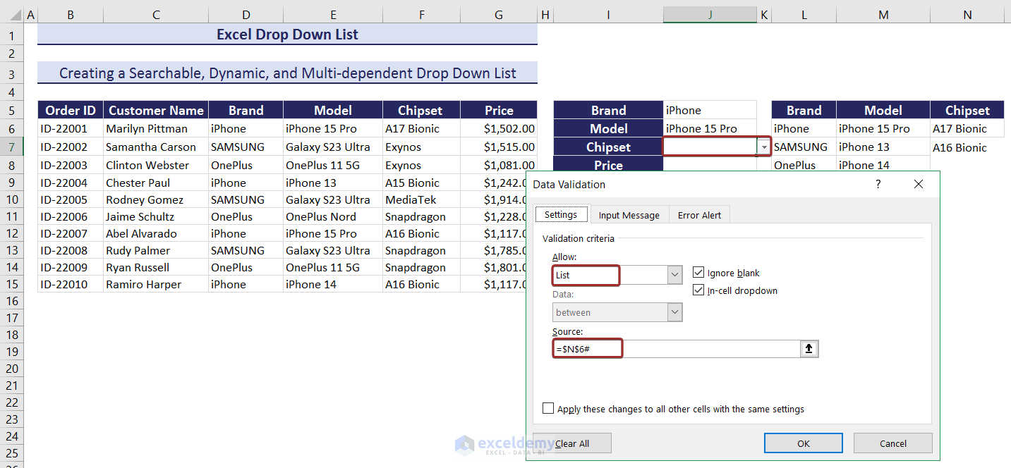
- Use the following formula in J8 to find the price of the product that matches the selected values.
=INDEX(G:G,MATCH(1,(J5=D:D)*(J6=E:E)*(J7=F:F),0))
As all drop-down lists are dynamic, you can add new entries and the drop-down lists will update.
12. Creating a drop-down List with a Custom Message
- Create a dependent drop-down list of the phone model, as described in Method 7.
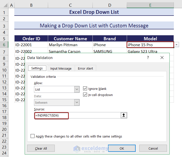
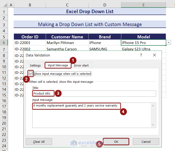
- In Data Validation, go to Input Message.
- Check Show input message when cell is selected.
- Set a title in Title and a custom message in Input message.
- Click OK.
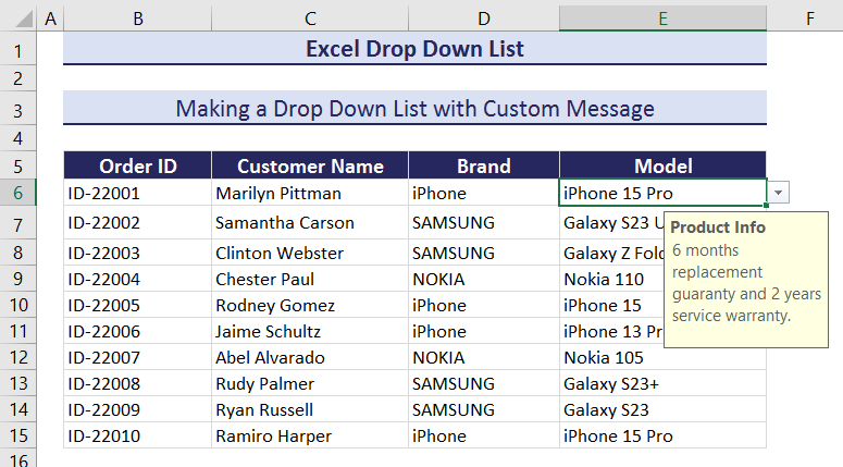
The custom message will be displayed when the cell is selected.
13. Creating an Editable drop-down List with an Error Alert Message
- Enter the following formula in G6 to create a dynamic column with unique brand names.
=UNIQUE(OFFSET(D6,0,0,COUNTA(D:D)-1,1))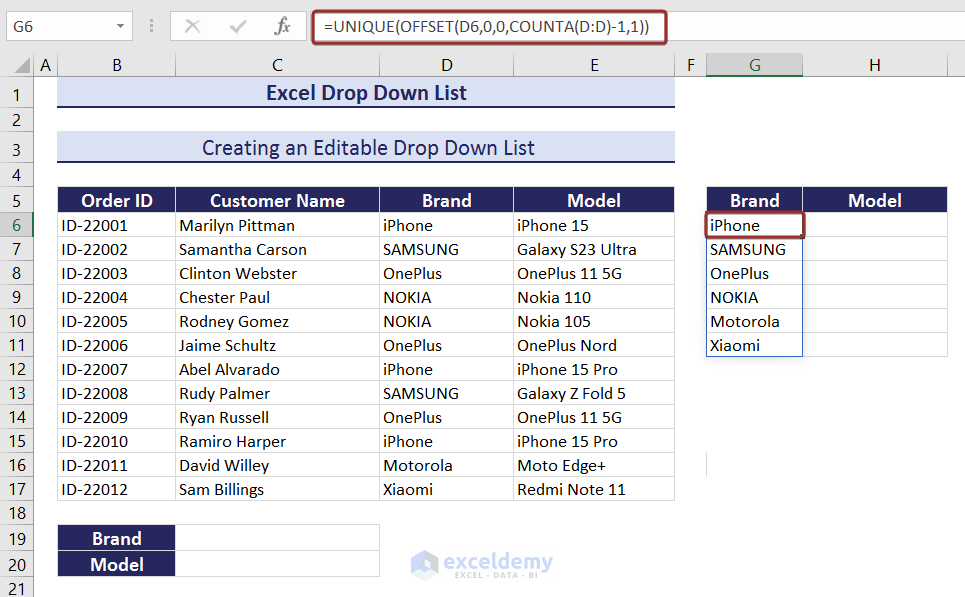
- Create a dynamic searchable drop-down list of brand names in C19 by entering the following formula in Source.
=$G$6#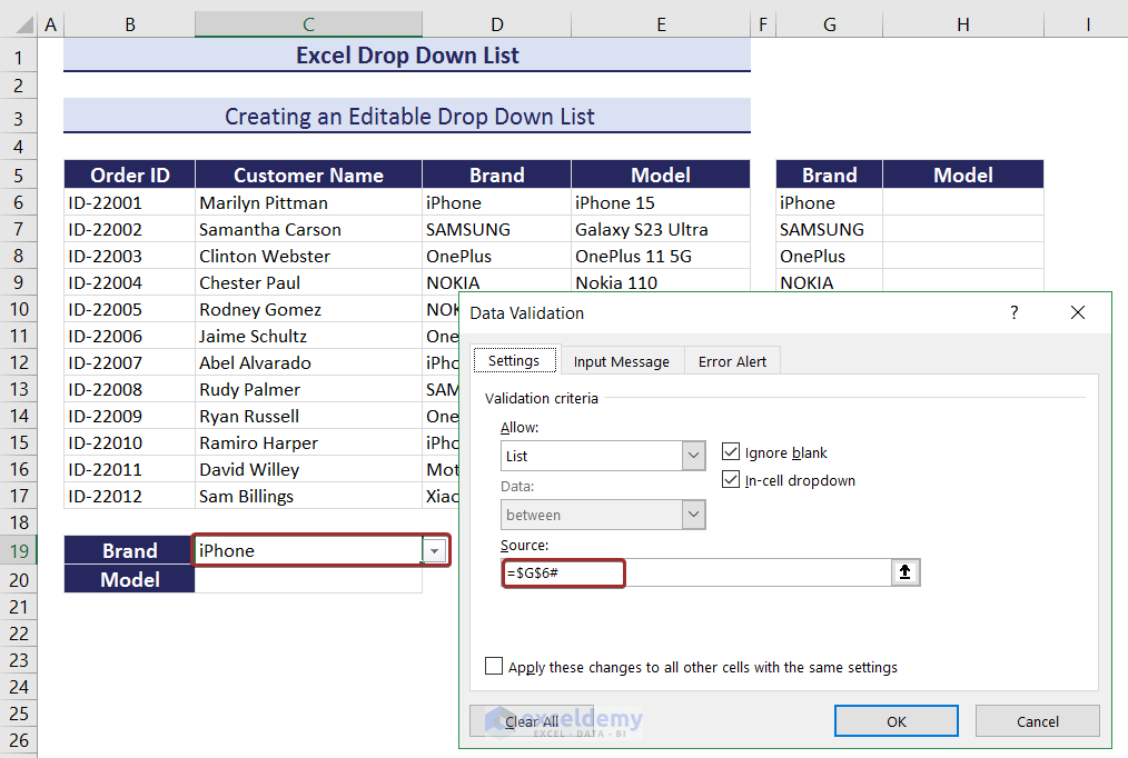
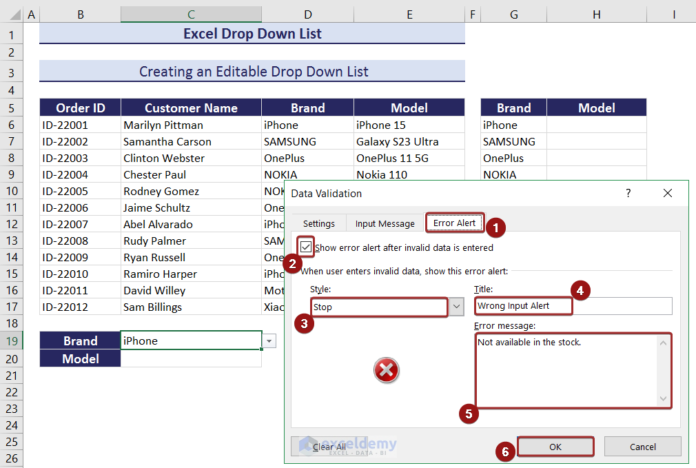
- To create a drop-down editable list, go to the Error Alert tab.
- Check the box Show error alert after invalid data is entered.
- Set a style, title, and error message for the wrong search value and click OK.
- Create a drop-down list with the values in Model.
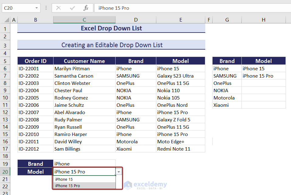
If you enter a wrong input in those editable drop-down lists, the error alert will be displayed with an option to retry or cancel.
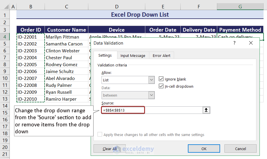
How to Add or Remove Items from an Excel drop-down List?
You can add or remove items by adding or removing cells while defining the range in Source.
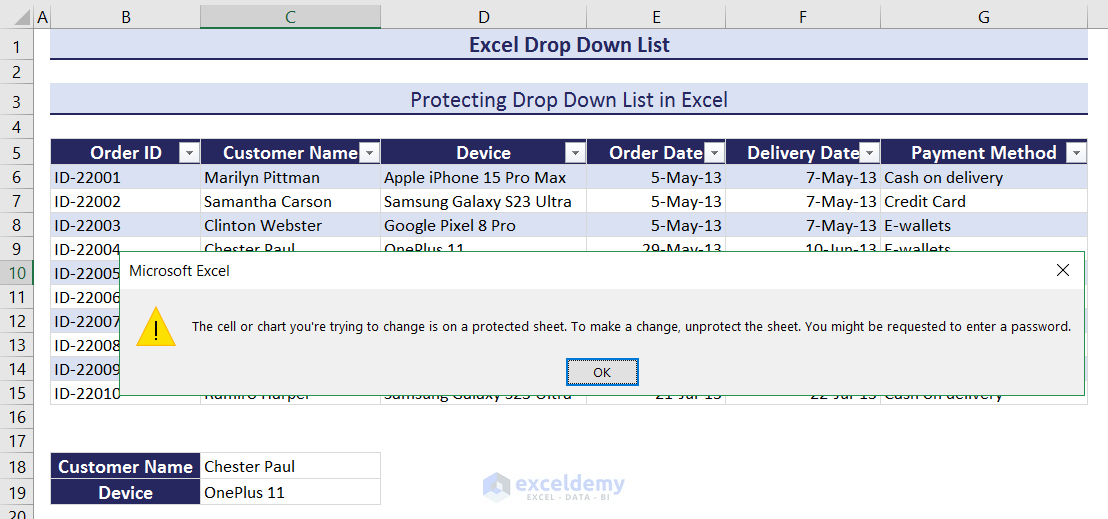
How to Protect a drop-down List in Excel?
A drop-down list of customer names was created in C18.
- Select the entire table and go to the Home tab.
- Click Alignment to extend it.
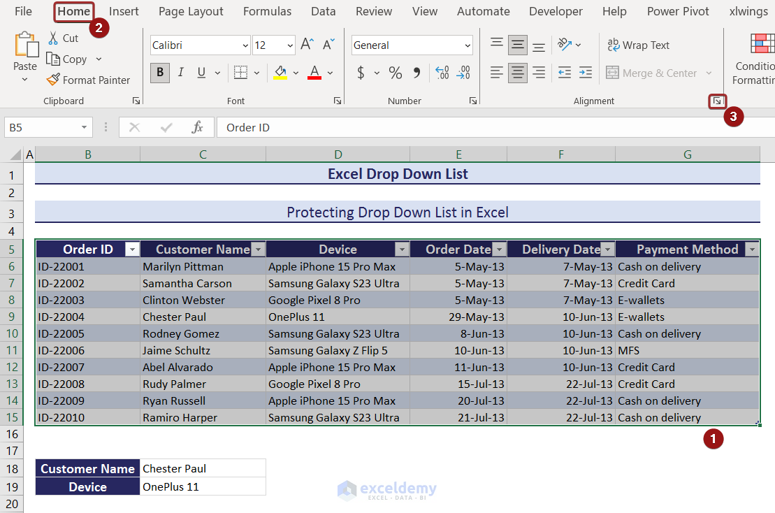
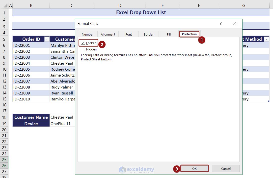
- In Format Cells, check Locked in the Protection tab.
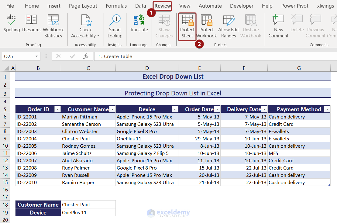
- The table is protected. Go to the Review tab and click on Protect Workbook.
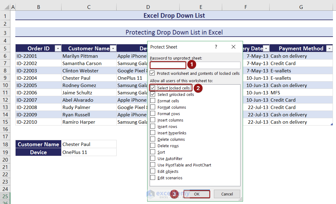
- Enter a password and check Select locked cells.
- Click OK.
- Re-enter the password.
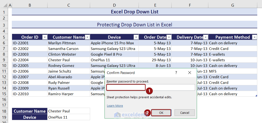
Both table and drop-down list are protected.
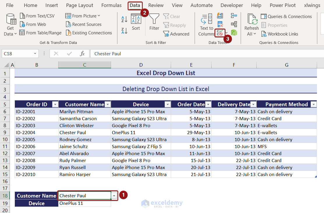
How to Delete a drop-down List in Excel?
- Select the drop-down list and go to the Data tab.
- Click Data Validation.
- In Data Validation, click Clear All.
- Click OK.
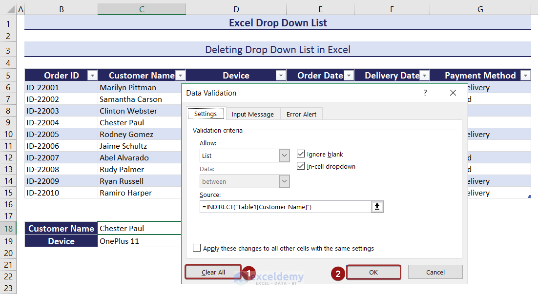
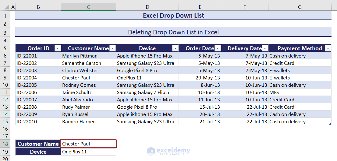
The drop-down list will be removed.
How to Filter a drop-down List & Extract Data Based on a Selection in Excel?
- Create a table.
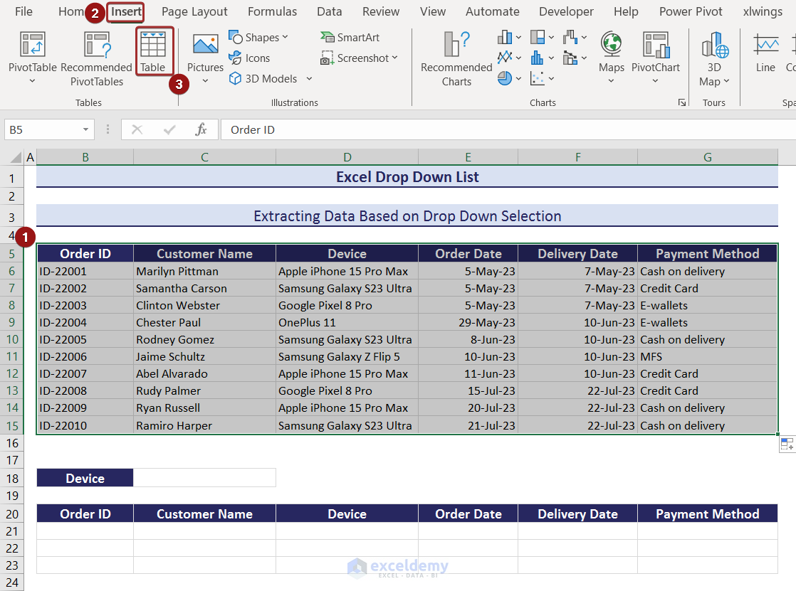
- Create a drop-down list in column D.
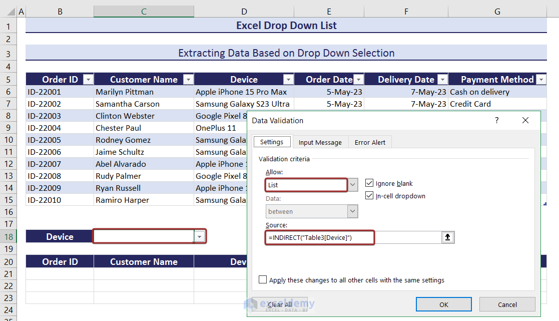
- Enter the following formula to extract the entire data based on the selection.
=FILTER(Table3,Table3[Device]=$C$18,"No Information Available")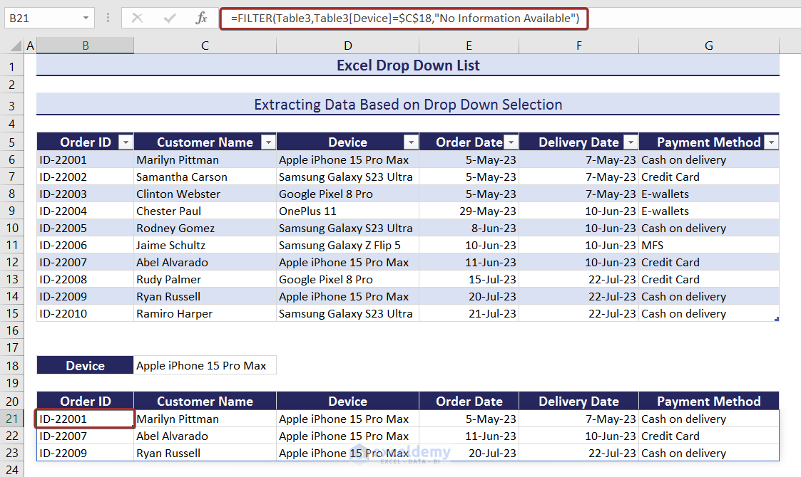
- Change the values of the drop-down list and data extraction will automatically be updated.
How to Solve Issues with an Excel drop-down List?
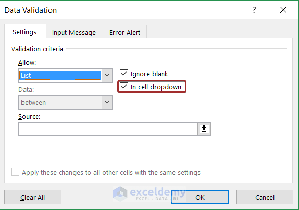
1. The drop-down List is Not Visible
Solution:
- Check In-cell dropdown to make the drop-down list visible.
2. Showing Blank in drop-down List
Solution:
- Define the drop-down list range to ignore blanks.
3. Valid Entries Not Allowed in drop-down List
Solution:
- Use proper cases while entering a valid entry.
4. Invalid Entries Allowed in drop-down List
As the source range is bigger than the actual value list, the values entered in those cells might be listed, even though they are invalid.
Solution:
- Define the drop-down list range to stop the entry of invalid elements.
Download Practice Workbook
Download the practice workbook.
Excel drop-down List: Knowledge Hub
- Create drop-down List in Excel
- Edit drop-down List in Excel
- drop-down List with Filter in Excel
- Excel Dependent drop-down List
- How to Remove drop-down List in Excel
- How to Link a Cell Value with a drop-down List in Excel
- Excel drop-down List Not Working
- IF Statement to Create Drop-Down List in Excel
- Extract Data Based on a drop-down List Selection in Excel
- Populate List Based on Cell Value in Excel
- drop-down List in Multiple Columns in Excel
- Blank Option to drop-down List in Excel
- Select from drop-down and Pull Data from Different Sheet
- [Fixed!] drop-down List Ignore Blank Not Working in Excel
- Autocomplete Data Validation drop-down List in Excel
<< Go Back to Data Validation in Excel | Learn Excel
Get FREE Advanced Excel Exercises with Solutions!
