Method 1 – Use the VLOOKUP Function to Select from a Drop-Down and Pull Data from a Different Sheet in Excel
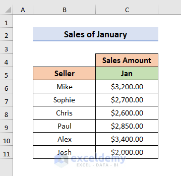
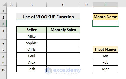
We will use a dataset that contains sales in three different months of some sellers in three different sheets.
- The sales in January are stored in the sheet named Jan.
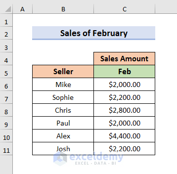
- The sales in February are stored in the sheet named Feb.
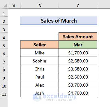
- Similarly, the sales in March are stored in the sheet named Mar.
Steps:
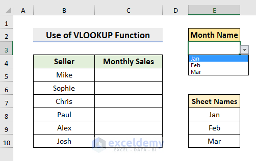
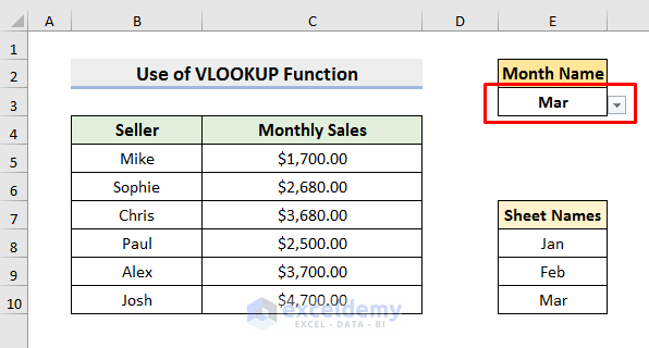
- Make a new sheet and create a structure of the dataset. We have created the structure of the dataset in a sheet named VLOOKUP function. We have written the Month Name as a lookup cell and Sheet Names in Column E.
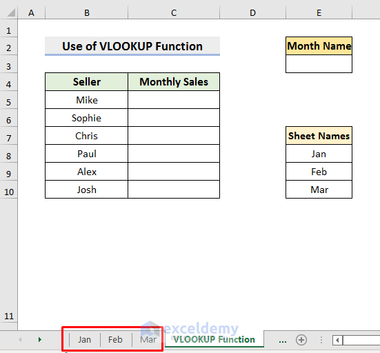
- Select Cell E3.
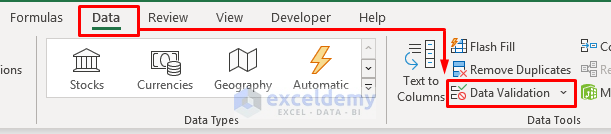
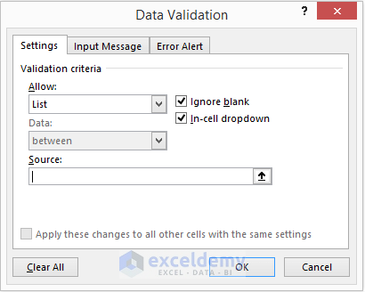
- Go to the Data tab and select the Data Validation option. It will open the Data Validation window.
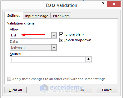
- Choose List in the Allow field and then select the Source field.
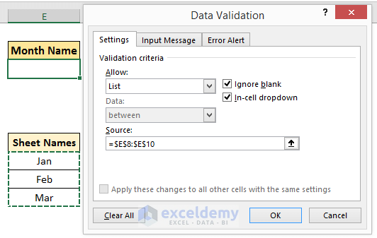
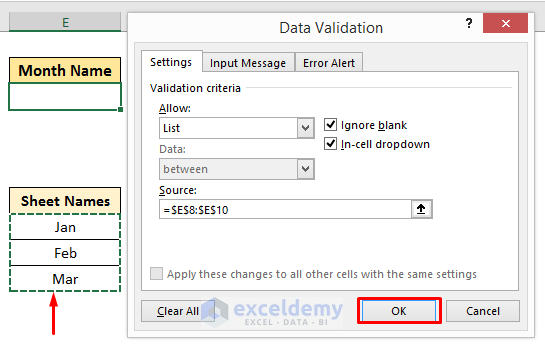
- Select the cells with months to add to the drop-down menu. We have used $E$8:$E$10.
- Click OK to proceed.
- You will see a drop-down menu in Cell E3. It will be used to choose the sheet.
- Select Cell C5 at first and copy this formula:
=VLOOKUP($B5,INDIRECT("'"&$E$3&"'!$B$5:$C$11"),2,FALSE)- Press Enter.
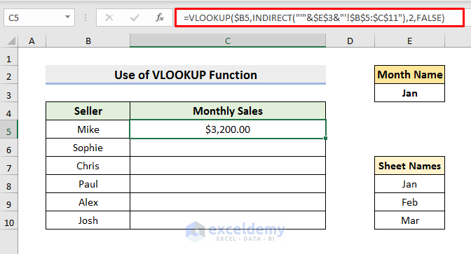
Here, we have used the INDIRECT function inside the VLOOKUP function.
How Does the Formula Work?
⇒ INDIRECT(“‘”&$E$3&”‘!$B$5:$C$11”)
The INDIRECT function returns a reference specified by a text string. Here, our argument refers to the text string stored in Cell E3. We have stored a sheet name in Cell E3. If you put Jan in Cell E3, it will return the B5:C11 range of the Jan sheet.
⇒ VLOOKUP($B5,INDIRECT(“‘”&$E$3&”‘!$B$5:$C$11”),2,FALSE)
This formula will look for the value stored in Cell B5 in the table array of the Jan sheet. Here, the column index number is 2 since that’s where the sales are listed, and we are looking for an exact match. So, we have used False at the end.
- Use the Fill Handle to see results in the rest of the cells.
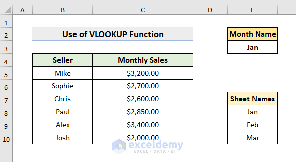
- If you change the Month Name using the drop-down menu, the dataset will be automatically updated.
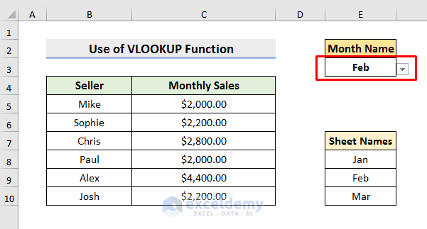
- We can also see the updated results for March.
Read More: Create a Searchable Drop Down List in Excel
Method 2 – Select from a Drop-Down and Pull Data from Different Sheet with the INDIRECT Function
Steps:
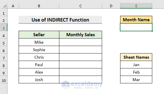
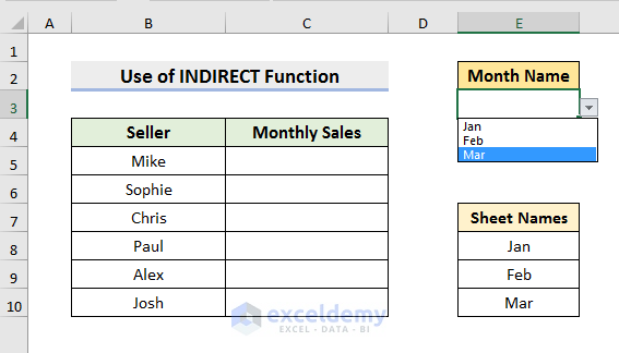
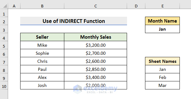
- Make a new sheet to put the results. We have created the structure of the dataset similar to the datasets in other sheets and written the lookup Month Name and Sheet Names in Column E.
- Go to the Data tab and select the Data Validation option. It will open the Data Validation window.

- Select List from the Allow field and then select the Source field.
- Select the range of options you want to add to the drop-down menu. We have selected cells E8 to E10, which contain the names of the sheets.
- Click OK to proceed.
- You will see a drop-down menu in Cell E3. You can choose the sheets from this drop-down menu.
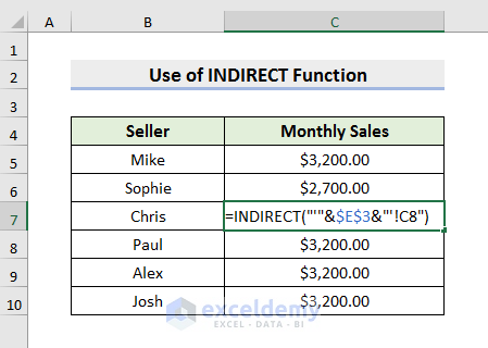
- Select Cell C5 and insert the following formula:
=INDIRECT("'"&$E$3&"'!C6")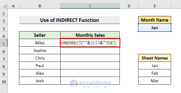
The INDIRECT function returns the reference specified by a text string. It has one compulsory argument. Our argument refers to the text string stored in Cell E3. We have stored a sheet name in Cell E3. Suppose, we have stored Jan in Cell E3. Then, it will return the Cell C6 of the Jan sheet.
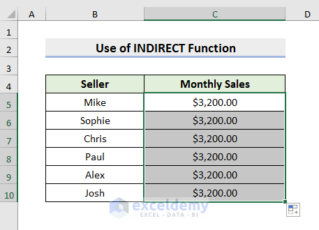
- Hit Enter and drag the Fill Handle to copy the same formula to the rest of the column.
- Select Cell C7 and write C7 instead of C6, then hit Enter.
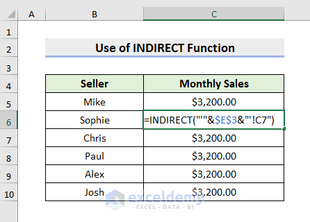
- Select Cell C8 and write C8 instead of C6, then hit Enter.
- Repeat for the rest of the cells with the appropriate row number and you will see results like below.
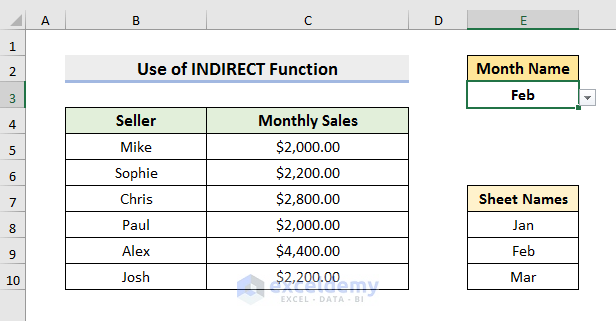
- If you change the Month Name using the drop-down menu, the dataset will be automatically updated.
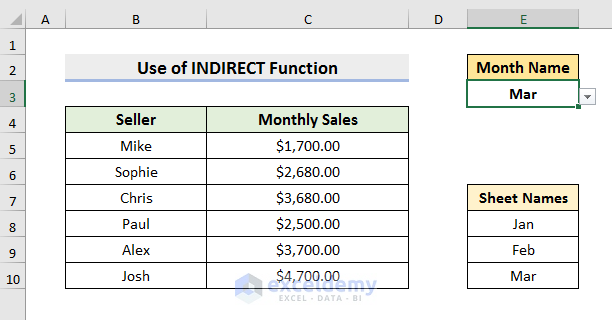
- We can also see the updated result for March.
Read More: How to Create Drop Down List in Multiple Columns in Excel
Method 3 – Choose from a Drop-Down and Extract Data from a Different Excel Sheet with the Data Validation Option
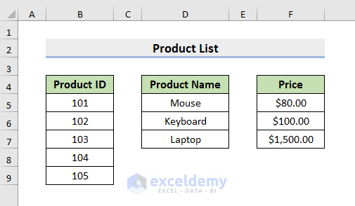
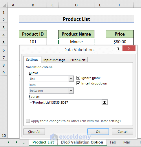
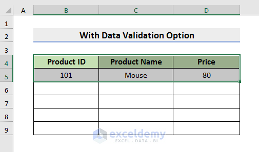
In this dataset, we have the ID, Name, and Price of some products. We will use this dataset to create a full dataset in another sheet. In this case, we will extract the data from our Product List dataset.
Steps:
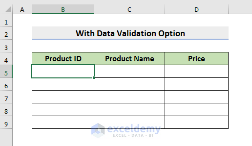
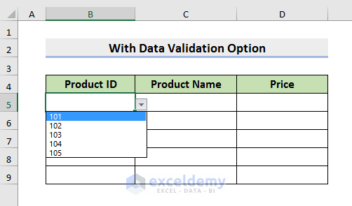
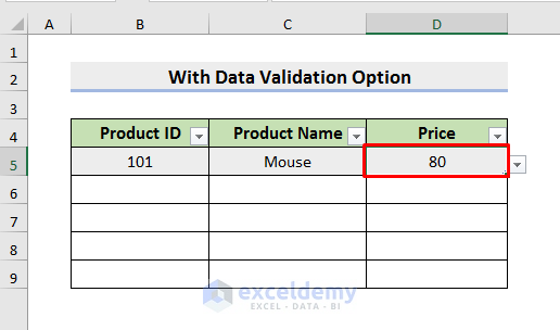
- Create the structure of the dataset and select Cell B5.
- Select the Data Validation option from the Data tab. It will open the Data Validation window.

- Select List from the Allow field.
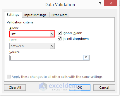
- Click on Source and choose the options you want to add to the drop-down menu by clicking the arrow at the end of the box.
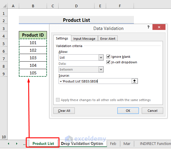
- Select the Product List sheet and use the ProductID column as the input array, or input the reference manually.
- Click OK to proceed.
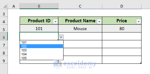
- You will see the Product ID in the drop-down menu in Cell B5.
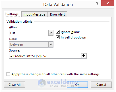
- Repeat the process for the drop-down menu in Cell C5. Choose the Product Name column from the Product List sheet as the source.
- For the drop-down menu in Cell D5, use the Price column the Product List sheet in the Data Validation source.
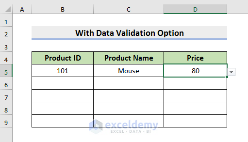
- You will see drop down menus in the desired cells of Row 5.
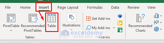
- Select rows 4 and 5.
- Go to the Insert tab and select Table.
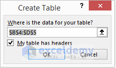
- The Create Table window will appear. Check My table has headers.
- Click OK to proceed.
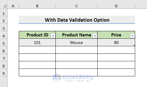
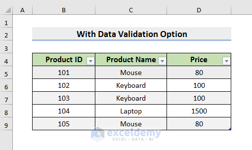
- You will see results like below.
- Select Cell D5.
- Press the Tab key. It will automatically include the drop-down menu in the cell in Row 6. You can fill the cells in the row using these drop-down menus.
- Follow the same process to insert the drop-down menu in every row and extract data using it.
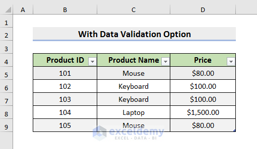
- You can change the Number Format to Currency in Column D to represent the dataset like below.
Read More: Creating a Drop Down Filter to Extract Data Based on Selection in Excel
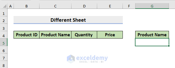
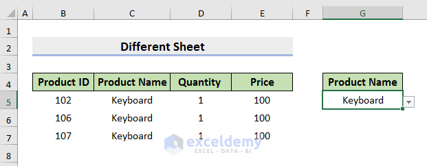
Method 4 – Select from a Drop-Down and Extract Data from a Different Sheet Using the FILTER Function in Excel
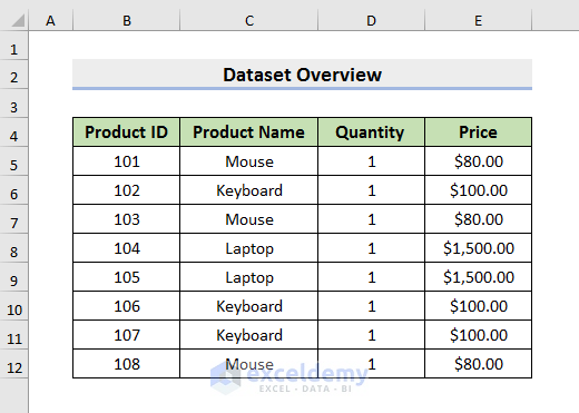
Here, we will use a dataset that contains the ID, Name, Quantity, and Price of some products.
Steps:
- Select any cell of your dataset. We have selected Cell B4 here.
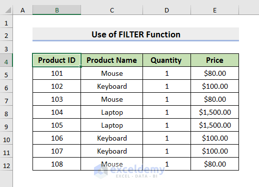
- Go to the Insert tab and select Table.

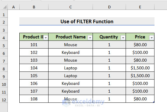
- Check My table has headers in the Create Table dialog box and click OK.

- The dataset will turn into a table like below.
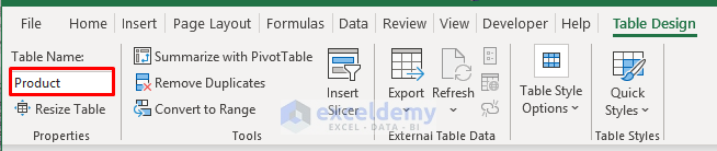
- Go to the Table Design tab and change the Table Name. We have named it Product.
- Go to a new sheet and select any cell. We have selected Cell I4.
- Insert the following formula:
=UNIQUE(Product[Product Name])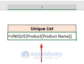
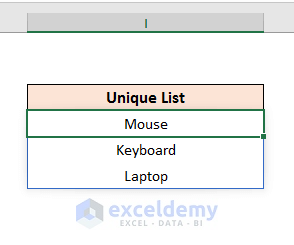
- Hit Enter to see the unique values in the Product Name column of the table.
Here, we have used the UNIQUE function. The UNIQUE function returns the unique values from a range or array. This formula returns the unique values from the Product Name column of the Product table.
- Go to the sheet where you have listed the unique values.
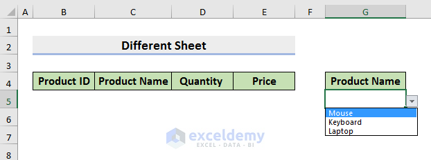
- Create the headers of the Product table in Row 4.
- Select Cell G5.
- Select the Data Validation option from the Data tab. It will open the Data Validation window.

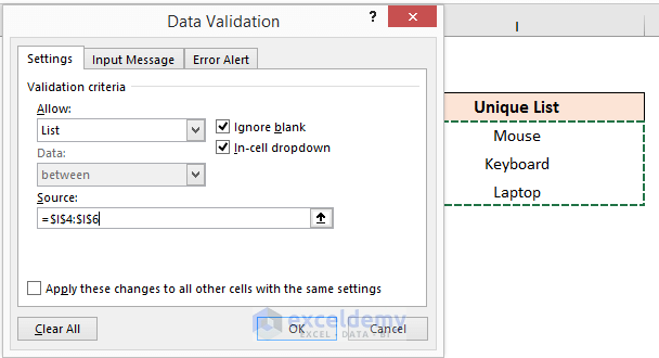
- Select List in the Allow field.
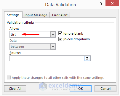
- For the Source, select Cells I4 to I6 (the list of unique values we output earlier).
- Click OK to proceed.
- You will see the drop-down menu in Cell G5.
- Select Cell B5 and copy the following formula:
=FILTER(Product,Product[Product Name]=G5)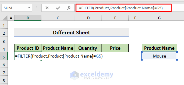
We have used the FILTER function to filter a range. The first argument is called the Product table. The second argument denotes that the Product Name will have to be the same as Cell G5.
- Hit Enter to see results like the below.
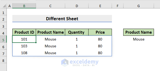
- If you change the product name using the drop-down menu, the dataset will automatically be updated.
Read More: How to Add Blank Option to Drop Down List in Excel
Things to Remember
- In Method 1, use the double quotation sign carefully while typing the formula. Otherwise, the result will be incorrect. Also, be extra careful with the column index number in the VLOOKUP Function.
- In Method 2, the formulas do not update automatically when you use the Fill Handle. To avoid this, edit the formula in each row.
- Method 3 is mainly used for creating a new dataset in a different sheet.
- Method 4 is applicable in Excel 365 only. For other Excel versions, use any other method.
Download Practice Book
Download the practice book here.
Related Articles
- How to Create a Form with Drop Down List in Excel
- How to Remove Used Items from Drop Down List in Excel
- How to Remove Duplicates from Drop Down List in Excel
- How to Fill Drop-Down List Cell in Excel with Color but with No Text
- [Fixed!] Drop Down List Ignore Blank Not Working in Excel
- How to Make Multiple Selection from Drop Down List in Excel
- How to Autocomplete Data Validation Drop Down List in Excel
- Hide or Unhide Columns Based on Drop Down List Selection in Excel
<< Go Back to Excel Drop-Down List | Data Validation in Excel | Learn Excel
Get FREE Advanced Excel Exercises with Solutions!
