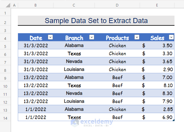
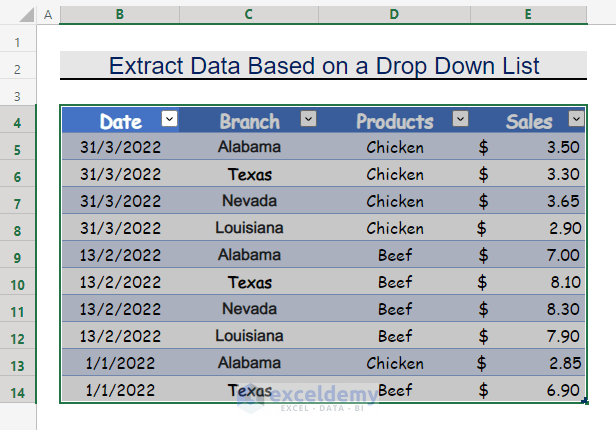
This is the sample dataset.
Step 1 – Create a Table to Extract Data Based on a Drop Down List in Excel
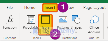
- Select the Table.
- Click Insert.
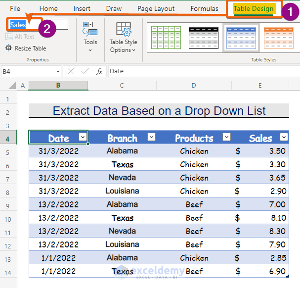
- Click Table Design, and name it (Sales).
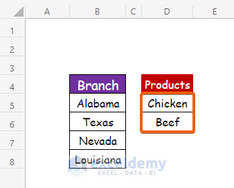
Step 2 – Extract Unique Data Based on a Drop Down List Selection
- To make a list with the unique Values in the Branch column, apply the UNIQUE function.
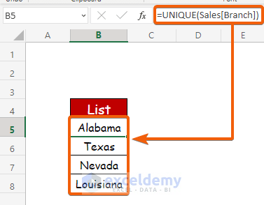
=UNIQUE(Sales[Branch])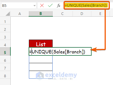
This is the output.
Read More: How to Create a Drop Down List with Unique Values in Excel
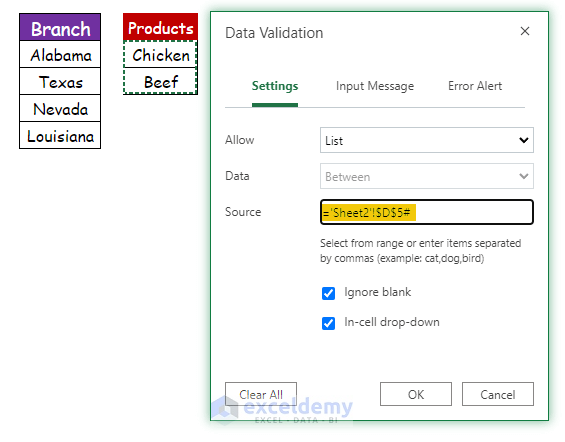
Step 3 – Insert a Data Validation List to Find Data Based on a Drop Down List in Excel
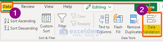
- To create a Data Validation list, click Data.
- Click Data Validation.
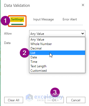
- Select List in Allow.
- Press Enter.
- In the source box, select List.
- Press Enter.
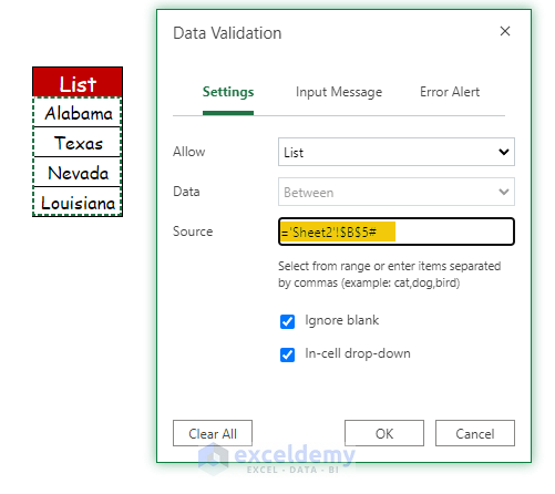
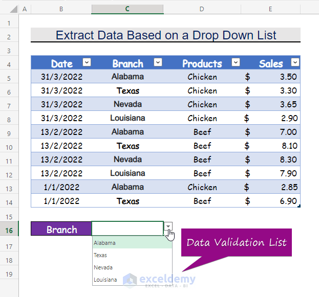
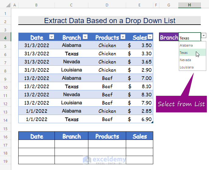
The Data Validation drop down list is created.
Read More: Creating a Drop Down Filter to Extract Data Based on Selection in Excel
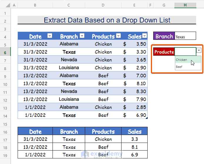
Step 4 – Apply the FILTER Function to Extract Data Based on a Drop Down List Selection in Excel
- In the FILTER Function, add the Table ‘Sales’ as the array element by using the formula.
=FILTER(Sales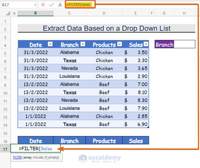
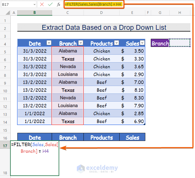
- In the Include argument, add the Branch.
- Use the following formula.
=FILTER(Sales,Sales[Branch] = H4- H4 is the cell of the drop-down selection box.
- In the ‘if empty’ argument, enter “Nothing Found”.
=FILTER(Sales,Sales[Branch] = H4,"Nothing Found")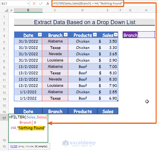
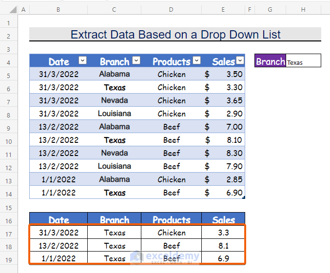
- Select any option (Texas), to extract all related value.
This is the output.
Notes. The FILTER function is only available in Microsoft 365.
Read More: Create Excel Filter Using Drop-Down List Based on Cell Value
Step 5 – Insert Another Criterion to Extract Data Based on a Drop Down List Selection
- Create a unique list with another column (Products). Enter the formula.
=UNIQUE(Sales[Products])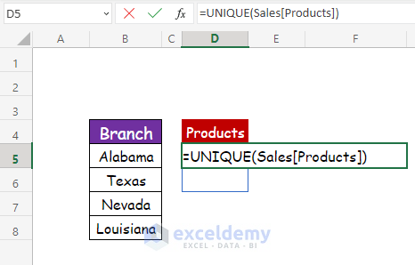
Another unique list will be created for the ‘Products‘ column.
- Create another Data Validation drop down list by selecting the cell values.
- Press Enter.
Step 6 – Extract Data Based on a Drop Down Selection List with Multiple Criteria
- After creating another drop-down list, this is the output.
- Enter the following formula to apply both the criteria.
=FILTER(Sales,(Sales[Branch] = H4)*(Sales[Products]=H6),"Nothing Found")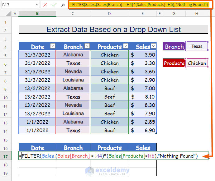
- Select two options from the two drop down lists.
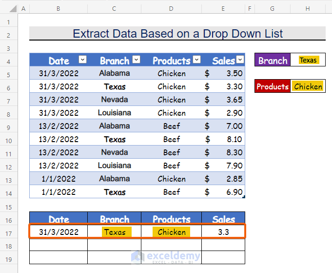
You will get the value of rows that meet both criteria.
Read More: How to Create Dependent Drop Down List with Multiple Words in Excel
Download Practice Workbook
Download this practice workbook to exercise.
Related Articles
- Conditional Drop Down List in Excel
- How to Use IF Statement to Create Drop-Down List in Excel
- How to Create Dynamic Dependent Drop Down List in Excel
- Excel Dependent Drop Down List
- How to Make Dependent Drop Down List with Spaces in Excel
- Excel Formula Based on Drop-Down List
- How to Populate List Based on Cell Value in Excel
- How to Change Drop Down List Based on Cell Value in Excel
<< Go Back to Excel Drop-Down List | Data Validation in Excel | Learn Excel
Get FREE Advanced Excel Exercises with Solutions!
