Here’s an overview of how you can use a drop-down list to affect other cells or create additional drop-down lists. Read on to learn how to make drop-down lists in Excel.
How to Create a Drop-Down List in Excel (Static and Dynamic)
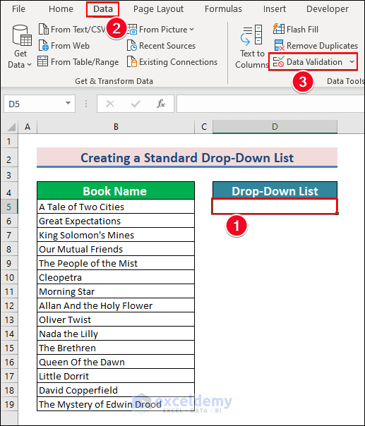
Case 1 – Creating a Static Drop-Down List Based on a Formula
Consider a dataset with a column Book Name. We need to make a drop-down list to select an item from this data.
- Select a cell where you want to make a list. We selected cell D5.
- Go to Data and click on Data Validation.
Data → Data Tools → Data Validation
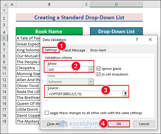
- In the Data Validation dialogue box, select List as the Validation criteria.
- In the Source field, apply the following formula:
=OFFSET($B$4,0,0,15)$B$4 is the Reference, 0s indicate the starting Row and Column, and 15 is the [height] of the OFFSET array.
- Click the OK button.
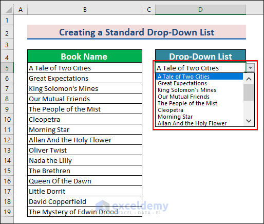
- You will get the formula-based drop-down list.
Read More: How to Populate List Based on Cell Value in Excel
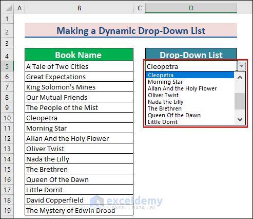
Case 2 – Making a Dynamic Drop-Down List Based on a Formula
The dynamic drop-down list allows you to auto-update your data. We will use the same datasheet.
- Insert a new Data Validation selector in the cell.
- In the Source field, apply the following formula:
=OFFSET($B$4,0,0,COUNTIF($B$4:$B$100,"<>"))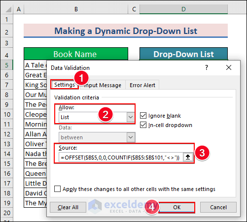
Formula Breakdown
- COUNTIF($B$4:$B$100,”<>”) is the [height] of the OFFSET function which counts the non-blank cells in the range B4:B100.
- 1st and 2nd 0 are the Rows and Columns to offset.
- $B$4 is the starting Reference of the OFFSET function.
- This creates a dynamic drop-down list.
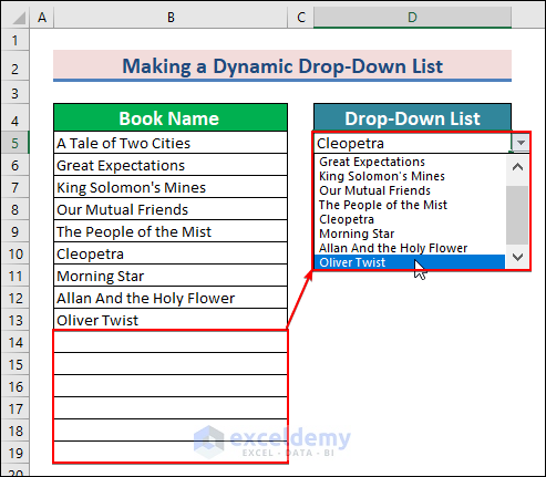
- Delete some data from your data list, and the drop-down list automatically updates.
Read More: How to Change Drop Down List Based on Cell Value in Excel
How to Use Excel Formulas Based on a Drop-Down List: 6 Handy Examples
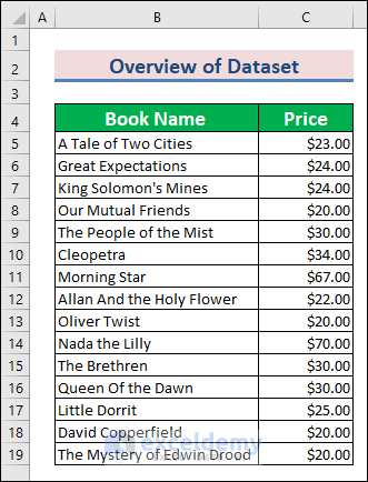
Let’s say we have a dataset where some books and their corresponding prices are given in columns B and C, respectively.
Method 1 – Use the Conditional IF Function Based on the Drop-Down List
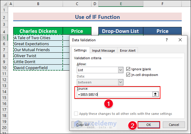
We have some books by Charles Dickens and the corresponding price names in the Price column. We will make the IF formula-based drop-down list to find the price of a chosen book.
- Create a drop-down list of the books.
- Select the table as your Source data.
- Click on OK.
- You will get a drop-down list.
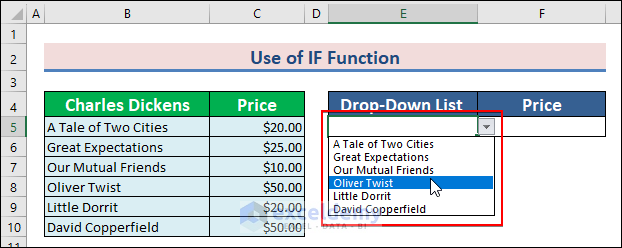
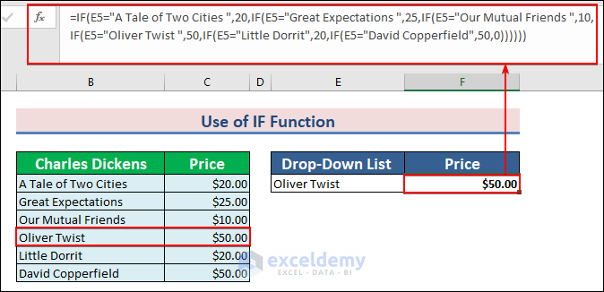
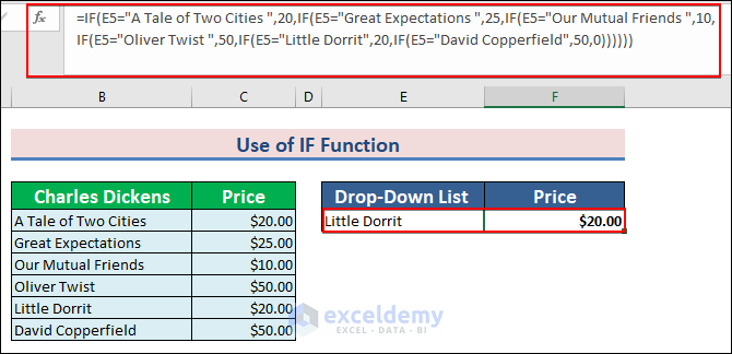
- Select cell F5 and copy the following formula in that cell, then hit Enter.
=IF(E5="A Tale of Two Cities ",20,IF(E5="Great Expectations ",25,IF(E5="Our Mutual Friends ",10,IF(E5="Oliver Twist ",50,IF(E5="Little Dorrit",20,IF(E5="David Copperfield",50,0))))))Where,
- E5(Data in the drop-down list) is the Logical_test.
- [Value_If_True] is the corresponding price of the book.
- [Value_If_False] then the function will move on to the next book and search for the match value.
- Change the source data to check the formula.
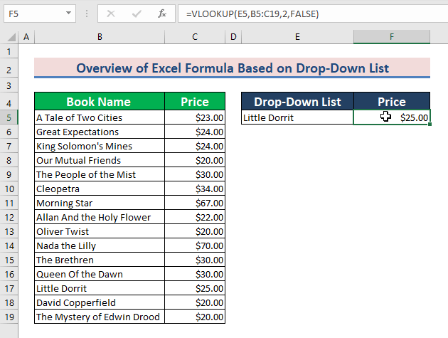
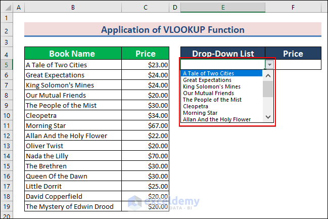
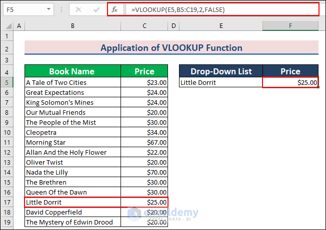
Method 2 – Apply the VLOOKUP Function to Fetch the Price of a Book Based on the Drop-Down
- Make a drop-down list in cell E5 using the Book Name column as the source.
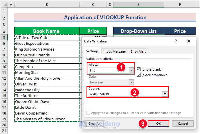
- Choose an item from the list.
- Insert the following formula in cell F5 and press Enter:
=VLOOKUP(E5,B5:C19,2,FALSE)Here, E4 (Data in the drop-down list) is the lookup_Value, B4:C18 is the table_Array, 2 is the col_index_num and FALSE is used to get the exact value.
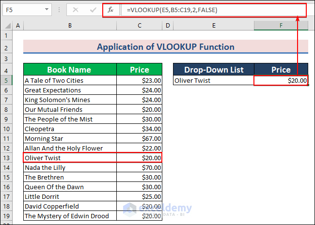
- You can change the source data in the drop-down list to check the formula.
Method 3 – Use a Dependent Drop-Down List Based on the INDIRECT Function
Consider this example where the Fruit and Vegetables columns are given with some data. We need to make a dependent list from that.
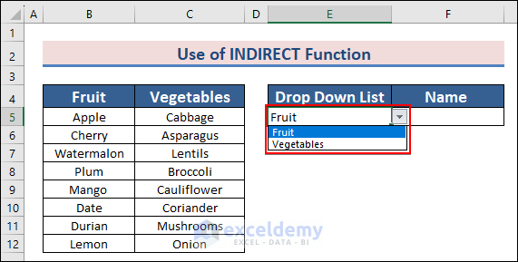
- Create a drop-down list with the column names (headers) as the source.
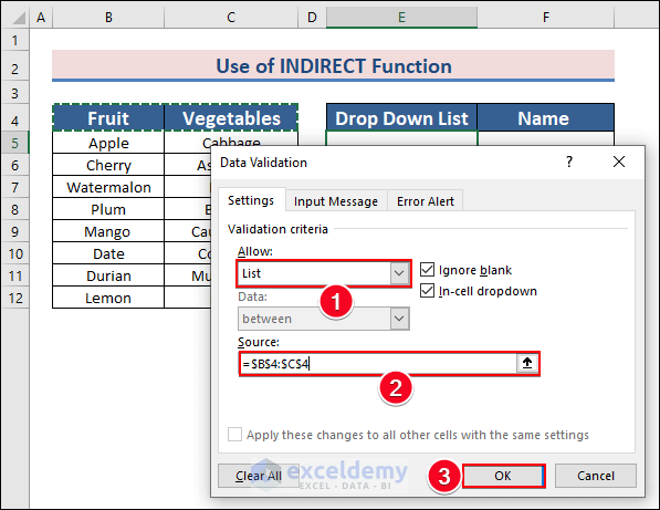
- We have the independent drop-down list for the columns.
- Select the Fruit and Vegetable columns (with headers), go to the Formulas tab, and click on Create From Selection.

- A new window pops up. Check Top Row and click Ok.
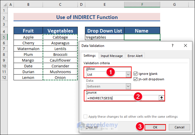
- Select cell F4 and make a new Data Validation drop-down list in it. In the Source box, apply this formula:
=INDIRECT(E5)When you select “Fruit” in the drop-down list (E4), this refers to the named range “Fruit” (through the INDIRECT function) and thus lists all the items in that category.
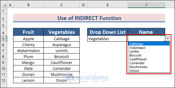
- Click OK. The formula-based dependent list is made.
- If you change Fruits to Vegetables, the list will show you options for vegetables from the dataset.
Read More: How to Create Dynamic Dependent Drop Down List in Excel
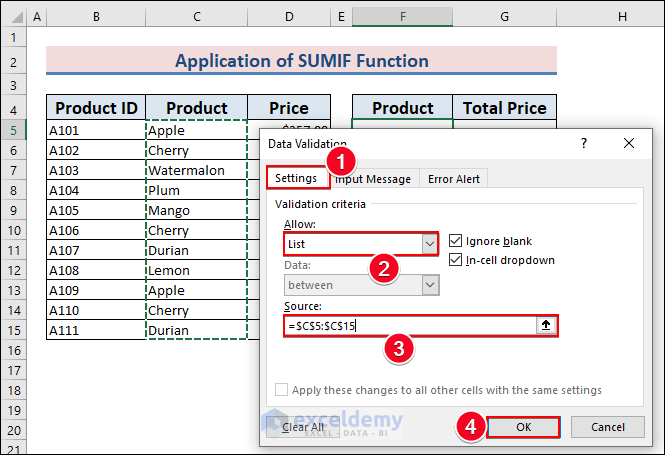
Method 4 – Apply the SUMIF Formula to Sum Values Based on the Drop-Down List
We will use the SUMIF function to calculate the total price of a particular product based on the drop-down list. We have some Product IDs, Product Names and Prices in columns B, C, and D respectively. Some product names repeat.
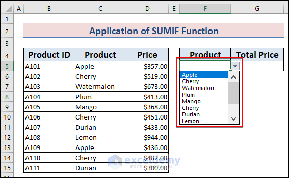
- Create a drop-down list in cell F5 using the Product column as the source.
- You will get a drop-down list for the selection. Let’s select Cherry.
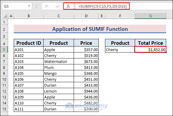
- Select cell G5 and copy the following formula in that cell, then hit Enter:
=SUMIF(C5:C15,F5,D5:D15)Here, C5:C15 is the range, F5 (Data in the drop-down list) is the criteria, and D5:D15 is the [sum_range] of the SUMIF function.
- You will get $1,452.00, which is the total price of Products named Cherry in the dataset.
Notes:
You can also use the SUMPRODUCT function to calculate the sum of values based on the selected option from a drop-down list.
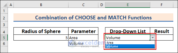
=SUMPRODUCT(SUMIF(C5:C15,F5,D5:D15))Method 5 – Combine CHOOSE and MATCH Functions to Calculate Geometry Parameters Based on the Drop-Down List
Let’s say we have the radius of a sphere. We will calculate the surface area or the volume of the sphere.
- Make a drop-down list in cell E5 with the Parameter column values as the source.
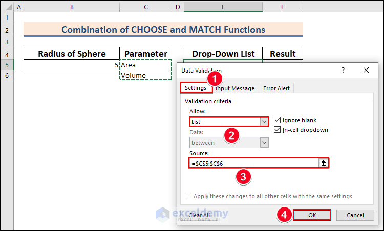
- Choose one of the options. We chose Volume.
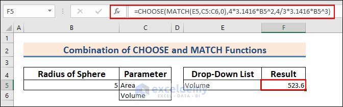
- Insert the following formula in cell G5 and press Enter:
=CHOOSE(MATCH(E5,C5:C6,0),4*3.1416*B5^2,4/3*3.1416*B5^3)- You will get 523.6, which is the approximate volume of a sphere with a radius of 5.
Formula Breakdown
- MATCH(E5,C5:C6,0) will match the value of the drop-down list (E5) in the range C5:C6 and returns 2.
- CHOOSE(MATCH(E5,C5:C6,0),4*3.1416*B5^2,4/3*3.1416*B5^3) will calculate the selected value from the drop-down list and returns 523.6 cubic units.
Method 6 – Use the FILTER Function Based on a Selection of a Drop-Down List
Consider a dataset where the Sales Representatives, State, Product, Quantity, and Sales columns are given. We will calculate the sales statements of a particular state, which we’ll choose via drop-down.
- Press Ctrl + T to create a table.
- Select data range $B$4:$F$24 and hit the OK option.
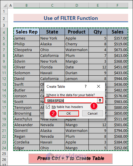
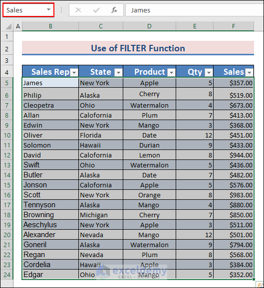
- Name the table as Sales.
- Open a new sheet and copy the below formula in cell B5.
=SORT(UNIQUE(Sales[State]))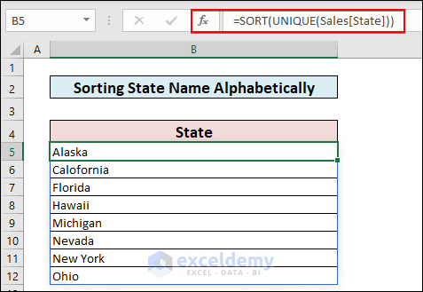
Formula Breakdown
- UNIQUE(Sales[State]) will find out the unique value of the state column from the Sales named range.
- SORT(UNIQUE(Sales[State])) will sort the unique value alphabetically.
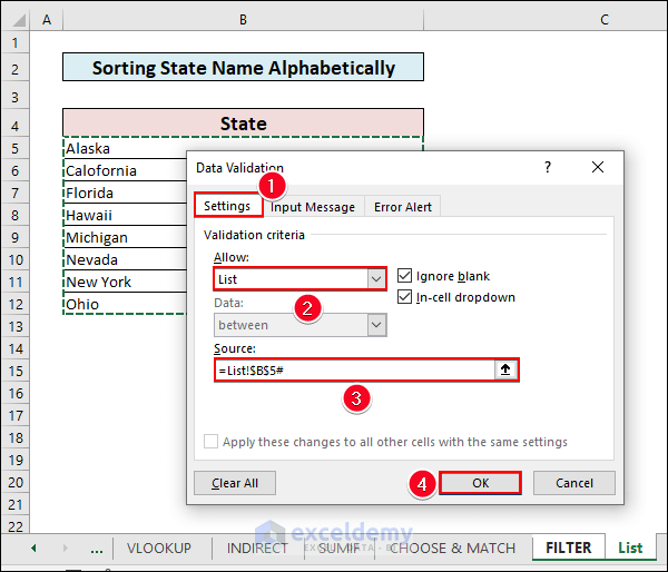
- Create a drop-down list in cell J5 using the previously made column as the source. You can put $B$5# as the source, since it’s a spill array. Don’t forget the worksheet reference.
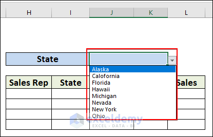
- This creates a drop-down list with values sourced from the column in a worksheet named List. Choose a state.
- Insert the following formula in cell H7 to find the sales statements of the chosen state from the drop-down list, then hit Enter:
=FILTER(Sales,Sales[State]=J4,"Not Found")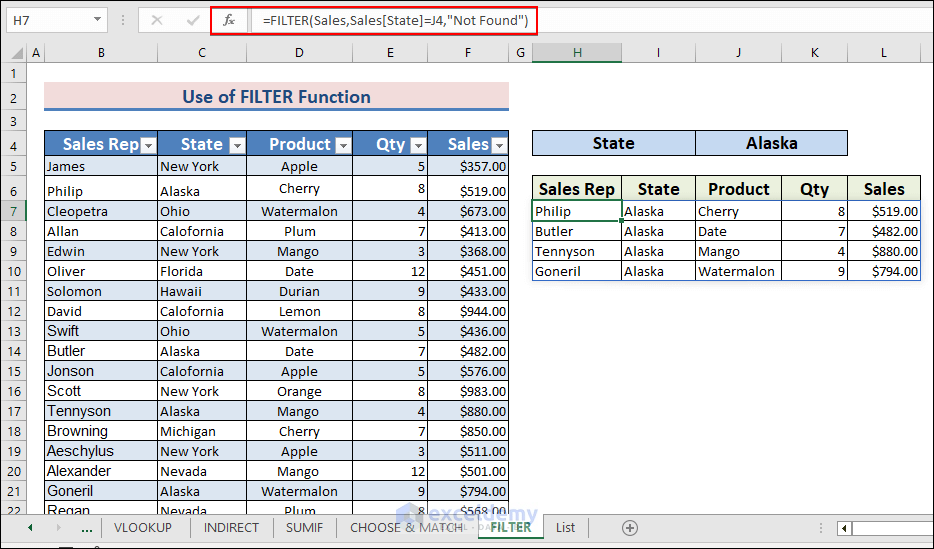
Read More: Create Excel Filter Using Drop-Down List Based on Cell Value
Things to Remember
- While creating a dynamic drop-down list, make sure that the cell references are absolute (such as $B$4) and not relative (such as B2, or B$2, or $B2)
- To avoid errors, remember to check “Ignore Blank” and “In-cell Dropdown”.
- Make sure to properly set up the drop-down list using the Data Validation feature in Excel. This will ensure that the list contains the correct options and that users can only select valid choices.
- When using a drop-down list in a formula, use the INDIRECT function to reference the selected option. This will allow the formula to dynamically update based on the user’s choice.
- The options in a drop-down list can be changed by editing the list source in the Data Validation dialog box. Make sure to update the list source if you add or remove options.
- You can use drop-down lists to populate cells with selected options or to filter data based on selected options.
Frequently Asked Questions
Can I use a formula in a drop-down list in Excel?
No, you cannot use a formula directly in a drop-down list in Excel. However, you can use a formula in a separate cell to calculate the options for the drop-down list and then refer to that cell as the source for the list.
How do I change the options in a drop-down list in Excel?
To change the options in a drop-down list in Excel, you need to first select the cell or cells where the drop-down list appears. Then, go to the Data tab in the ribbon and click on Data Validation. In the Data Validation dialog box, select List as the validation criteria and edit the options in the Source field.
Can I use a drop-down list to filter data in Excel?
Yes, you can use a drop-down list to filter data in Excel. To do this, you need to first create the drop-down list and then select the cell or cells that contain the data you want to filter. Then, go to the Data tab in the ribbon and click on Filter. In the filter drop-down menu, select Filter by Selected Cell’s Value and choose the cell that contains the drop-down list.
Download Practice Workbook
Downloads this workbook to practice while reading this article.
Related Articles
- Conditional Drop Down List in Excel
- Excel Dependent Drop Down List
- How to Make Dependent Drop Down List with Spaces in Excel
- How to Create Dependent Drop Down List with Multiple Words in Excel
- How to Extract Data Based on a Drop Down List Selection in Excel
<< Go Back to Excel Drop-Down List | Data Validation in Excel | Learn Excel
Get FREE Advanced Excel Exercises with Solutions!
