How to Create an Excel Filter Using a Drop-Down List Based on the Cell Value

Step 1 – Set up a Unique List to Create a Drop-Down List Filter Based on the Cell Value in Excel

Copy the data. Here, the data in the Category column.
Select the data and go to DATA > Remove Duplicates.

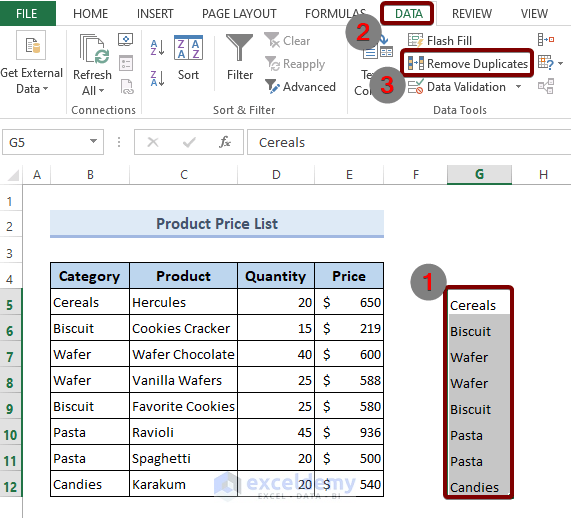
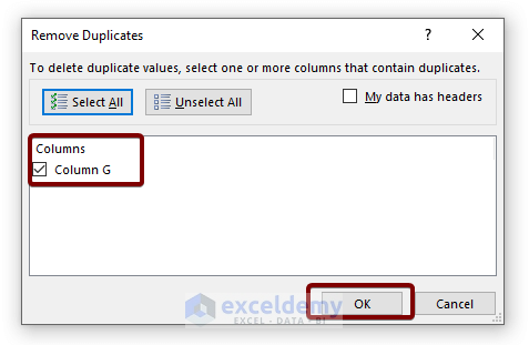
In the Remove Duplicates dialog box, click OK.

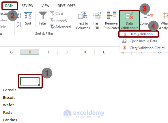
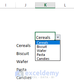
The list of unique items is created. To add the drop-down list:

Select a cell and go to DATA > Data Validation > Data Validation.

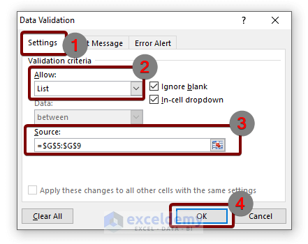
In the Data Validation dialog box:

In Settings, select List in Allow.
Enter the cell range in Source.
Click OK.

This is the output.

Step 2 – Prepare the Drop Down List to Filter data

Insert 3 helper columns: Row SL, Matched, and Ordered.

The First Helper Column: .

Use the Row SL column to store the serial number of the rows in the data table:

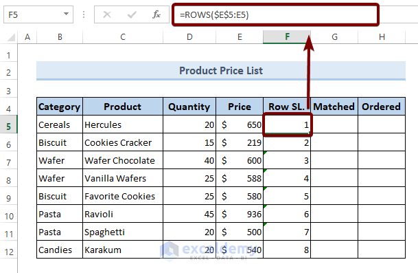
Enter the following formula in F5.

=ROWS($E$5:E5)

The argument for the ROWS function is an array:

$E$5 is the first cell in Row SL. Add a dollar sign by pressing F4 to lock the cell address.
E5 is also the first cell in Row SL.

The formula calculates the difference between $E$5 and E5. As you drag the Fill Handle icon from F5 to F12, $E$5 is locked but E5 changes. The distance between the two cell addresses increases and you get the serial numbers of the row.

Press ENTER.
Drag down the Fill Handle to see the result in the rest of the cells.

The Second Helper Column: Matched

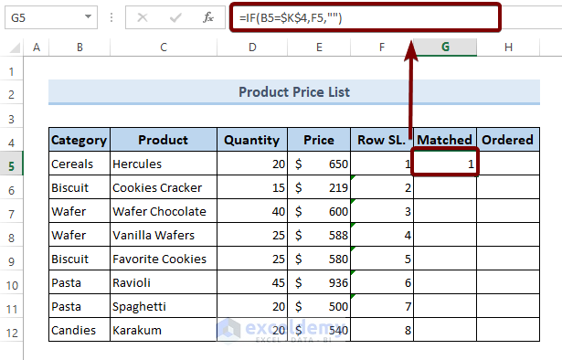
Use this column to return the serial number of rows that match the item selected in the drop-down list in K4:

Use the following formula in G5.

=IF(B5=$K$4,F5,"")

In the formula,

B5 is the cell address of the first item to match with the selected item of the drop-down list.
$K$4 is the cell address of the drop-down list.
F5 is the cell address of the value to return if there is a match between B5 and $K$4.
“” is used to return a blank if there are no matches between B5 and $K$4.

Press ENTER.
Drag down the Fill Handle to see the result in the rest of the cells.

The Third Helper Column: Ordered

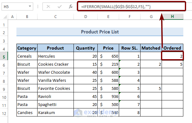
Use this column to see row numbers in one cell after another:

In H5, use the following formula:

=IFERROR(SMALL($G$5:$G$12,F5),"")

$G$5:$G$12 is the cell range in which the SMALL function will look for the smallest number.
F5 helps the SMALL function find the smallest numbers sequentially, as it contains 1, and the number increases by 1 when you drag the Fill Handle.
“” is used to keep a cell blank with the help of the IFERROR function, if an error occurs.

Press ENTER.
Drag down the Fill Handle to see the result in the rest of the cells.

Step 3: Use the Drop-Down List to Filter data

Copy the data table to another location.
Clear the content using the Clear Contents command. You can also select the table and press DELETE.
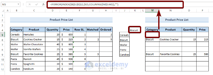
In the first cell of the copied table, use the following formula:

=IFERROR(INDEX($B$5:$E$12,$G5,COLUMNS($M$5:M5)),"")

$B$5:$E$12 is the cell range of the original data table.
$G5 is the first cell of the second helper column.
$M$5:M5 is the cell range of the first column of the copied data table.
“” is used to leave all cells blank with the help of the IFERROR function if data is unavailable for the selected item in the drop-down list filter.

Press ENTER.
Drag down the Fill Handle to see the result in the rest of the cells.

Download Practice Workbook

Download the Excel file.

Filter with Drop-Down List.xlsx

<< Go Back to Excel Drop Down List Filter | Excel Drop-Down List | Data Validation in Excel | Learn Excel

Get FREE Advanced Excel Exercises with Solutions!

How to Create an Excel Filter Using a Drop-Down List Based on the Cell Value – 3 Steps