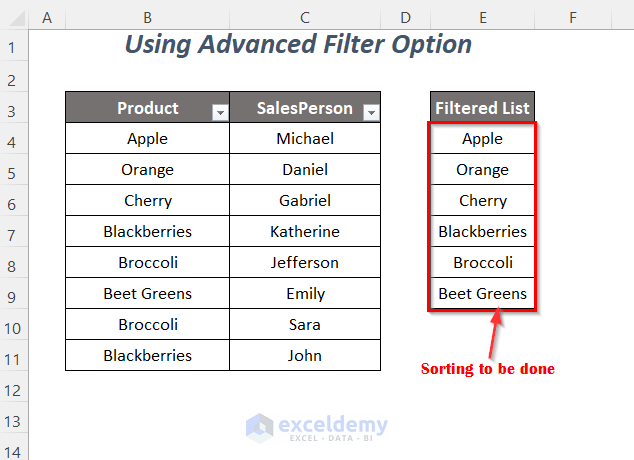
Method 1 – Using an Advanced Filter Option to Copy a Filter Drop-Down List
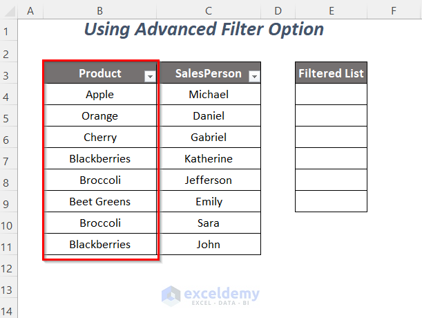
We have the products listed in the Product column, but the products are not sorted properly, and some duplicate products, like Blackberries and broccoli, remain there.
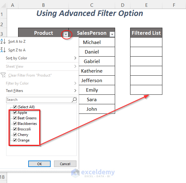
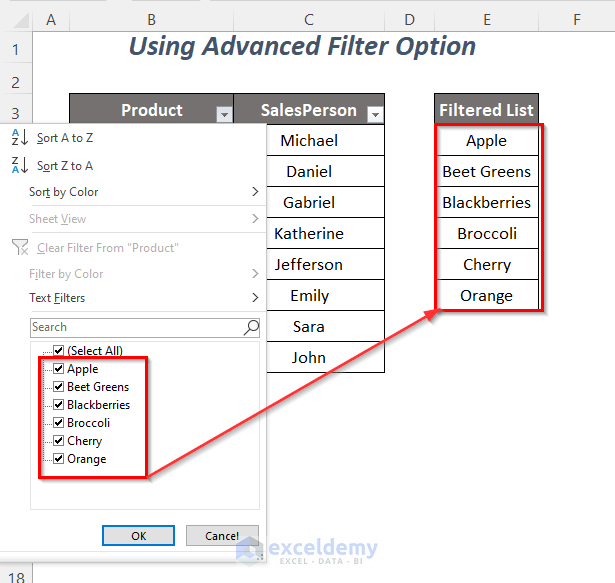
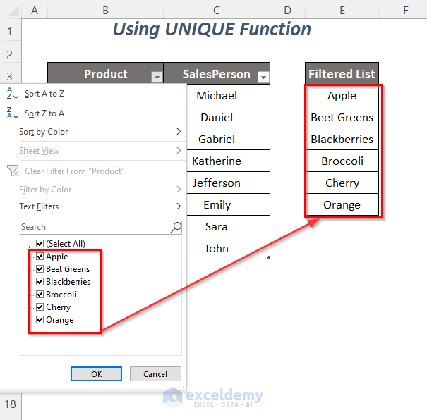
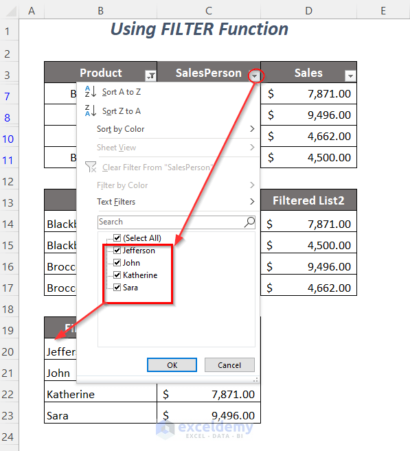
When we click on the filter dropdown symbol, we get the list sorted from A to Z, and there is no duplicate value. Our task is to copy this dropdown list to the Filtered List column, and we will do it using the Advanced Filter option.
Steps:
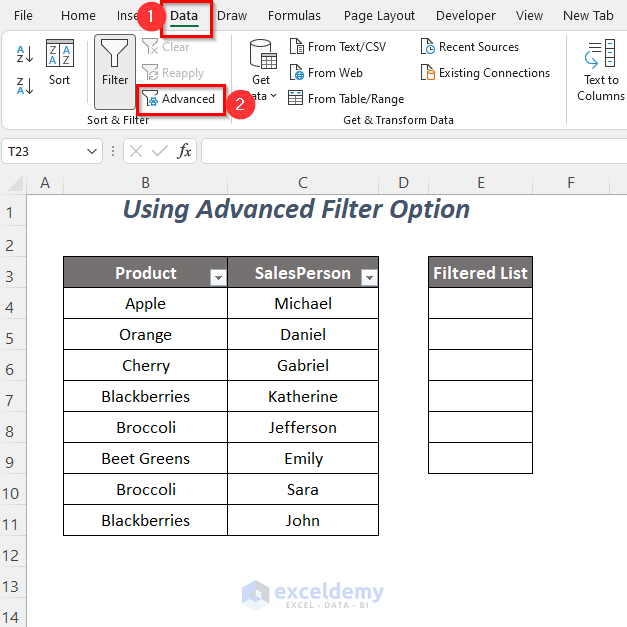
- Go to the Data Tab and the Sort & Filter Group, then select the Advanced Option.
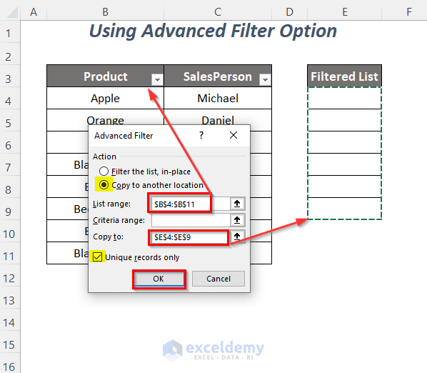
- The Advanced Filter wizard will open up.
- Check the options Copy to another location and Unique records only.
- Select the products as a List range and the destination range where you want the outputs in the Copy to box.
- Press OK.
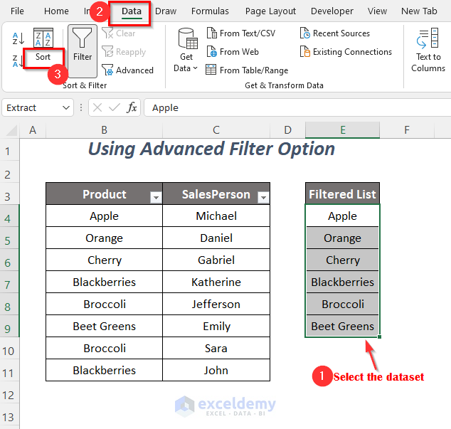
The list of unique products is in the Filtered List column but has not yet been sorted.
- Select the dataset and go to the Data Tab >> Sort & Filter Group >> Sort Option.
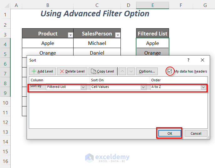
- The Sort wizard will pop up,
- Select Sort by → Filtered; List Sort On → Cell Values; Order → A to Z.
- Click on the My data has headers option and press OK.
The Filtered List is sorted, and the filter dropdown list is copied in the Filtered List column.
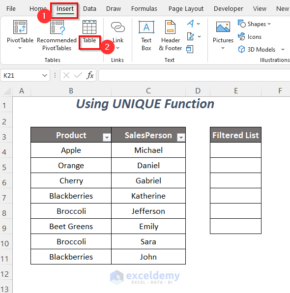
Method 2 – Using the UNIQUE Function to Copy a Filter Drop-Down List
Steps:
- To convert the range into a table,
- Go to the Insert Tab and select the Table Option.
- The Create Table wizard will appear.
- Select the range and click on the My table has headers option.
- Press OK.
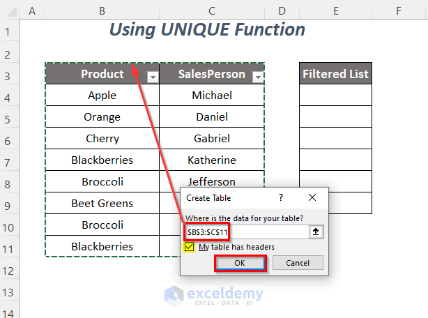
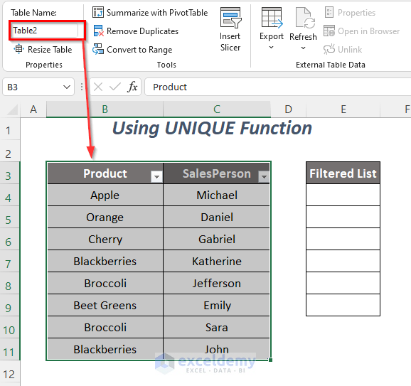
Table2 will be created.
- Enter the following function in cell E4 to get the unique values from the Product column.
=SORT(UNIQUE(Table2[Product],FALSE,FALSE))Here, Table [Product] is the range of the Product column of Table, The first FALSE is for Return unique rows, and the second one is for Return every distinct item. Then UNIQUE will give us the list of unique products, and then it will be sorted out by the SORT function.
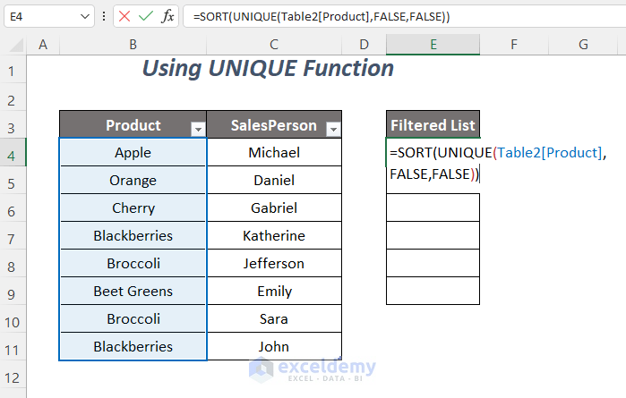
- Press ENTER to get the filter dropdown list of the Product column in the Filtered List column.
The UNIQUE function is only available for Microsoft Excel 365 version.
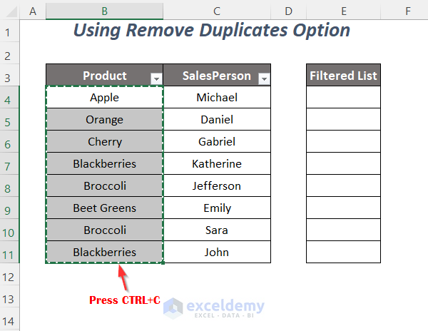
Method 3 – Using the Remove Duplicates Option to Copy a Filtered Drop-down List
Steps:
- Select the range of the Product column and press CTRL+C.
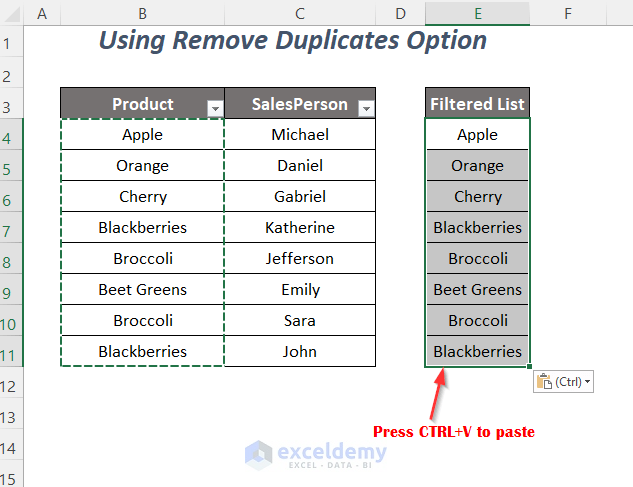
- Press CTRL+V to paste the list in the Filtered List column.
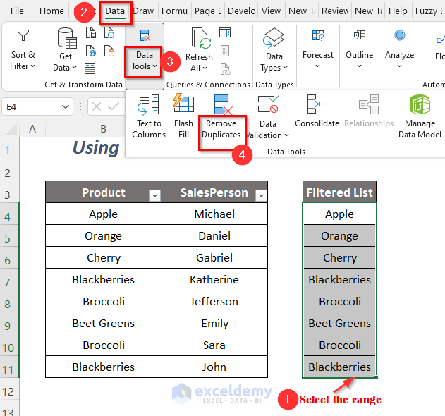
To get the unique values by removing the duplicates,
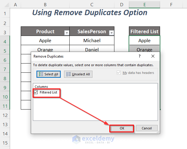
- Select the data range and go to the Data Tab >> Data Tools Group >> Remove Duplicates Option.
- The Remove Duplicates dialog box will appear.
- Check the Filtered List option and press OK.
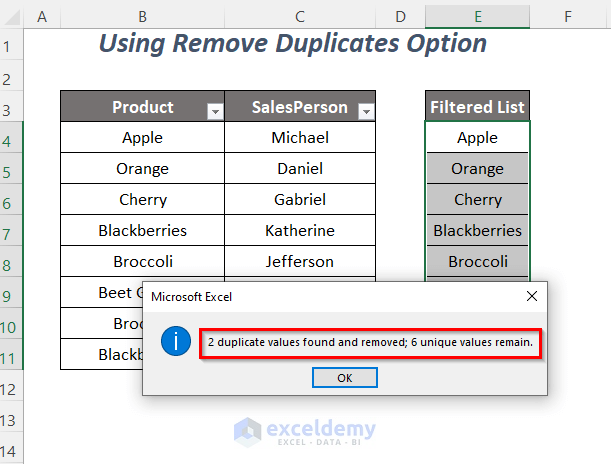
You will get a message box saying it has removed 2 duplicate values.
- Press OK.
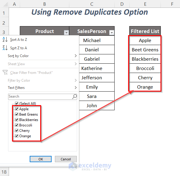
After sorting the texts from A to Z like Method-1 we will get the filter dropdown list of the Product column in the Filtered List column.
Read More: How to Remove Duplicates from Drop-Down List in Excel
Method 4 – Using the FILTER Function to Copy and Filter a Drop-Down List
4.1: Using the FILTER Function
Steps:
- Enter the following formula in cell B14:
=FILTER(B7:D11,B7:B11=B7," ")Here, B7:D11 is the range, then FILTER will search for the value Blackberries of cell B7 in the range B7:B11=B7, and for empty cells, it will return a blank.
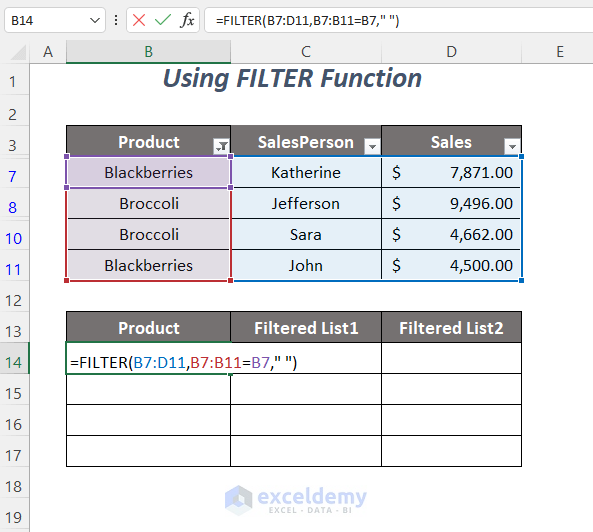
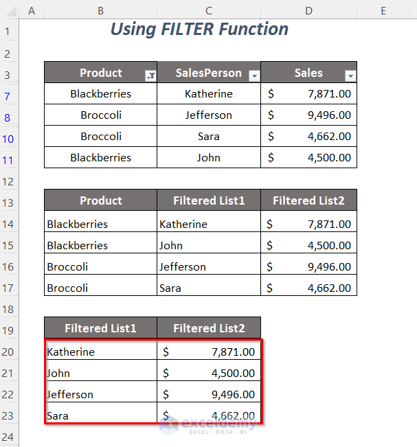
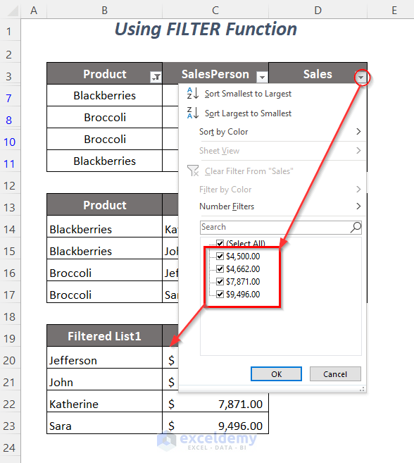
- Press ENTER. We will get the salespersons’ names and the sale values for the product Blackberries.
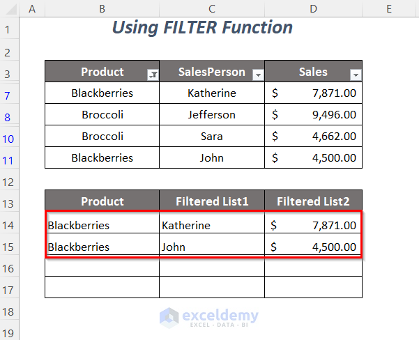
To extract the values for the product, Broccoli,
- Enter the following formula in cell B16:
=FILTER(B7:D11,B7:B11=B8," ")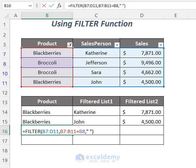
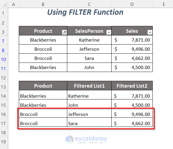
- Press ENTER, and you will get the salespersons’ names in the Filtered List1 column and the sales values in the Filtered List2 column.
The FILTER function is only available for the Microsoft Excel 365 version.
4.2 Copying the Values and Sorting them
Steps:
- Copy the lists by pressing CTRL+C.
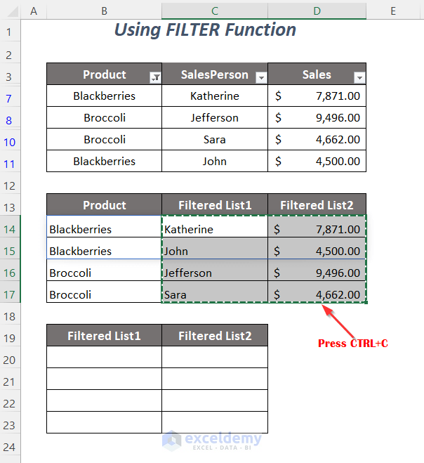
- Select the cell where you want to paste them.
- Right-click here, and select the option Paste Values.
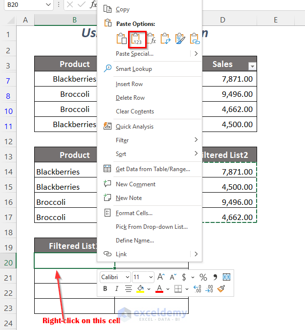
We will get the values of the Filtered List1 and Filtered List2 in the following dataset.
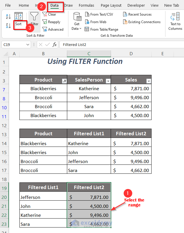
To sort the salespersons’ names from A to Z and the sales values from lowest to highest values,
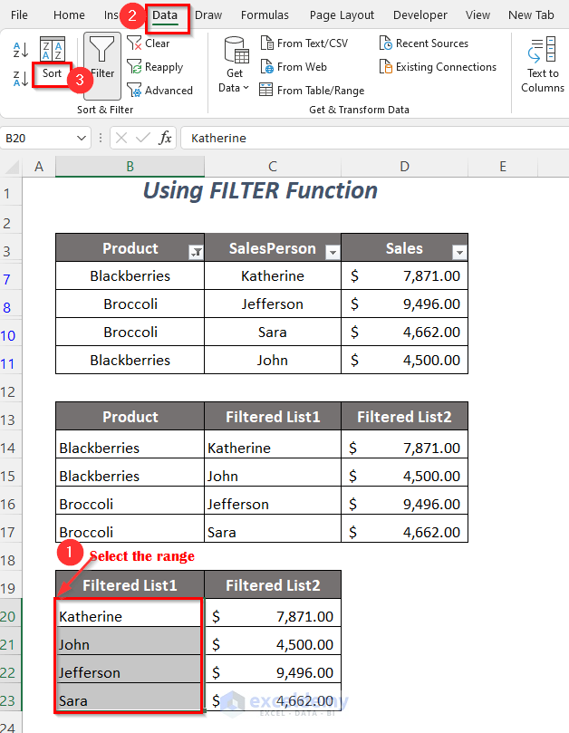
- Select the range of the Filtered List1 column.
- Go to the Data Tab >> Sort & Filter Group >> Sort Option.
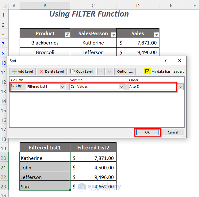
The Sort dialog box will pop up.
- Select the following: Sort by → Filtered List1; Sort On → Cell Values; Order → A to Z.
- Click on the My data has headers option and press OK.
The values of Filtered List 1 will be sorted now, and we will now work with the sales values of the Filtered List2 column.
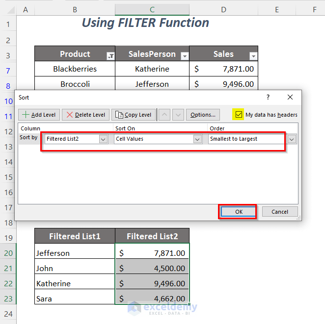
- Select the range of the Filtered List2 column.
- Go to the Data Tab >> Sort & Filter Group >> Sort Option.
The Sort dialog box will appear.
- Select the following: Sort by → Filtered List2; Sort On → Cell Values; Order → Smallest to Largest.
- Click on the My data has headers option and press OK.
We have sorted the values of the Filtered List1 and Filtered List2 columns as we wanted.
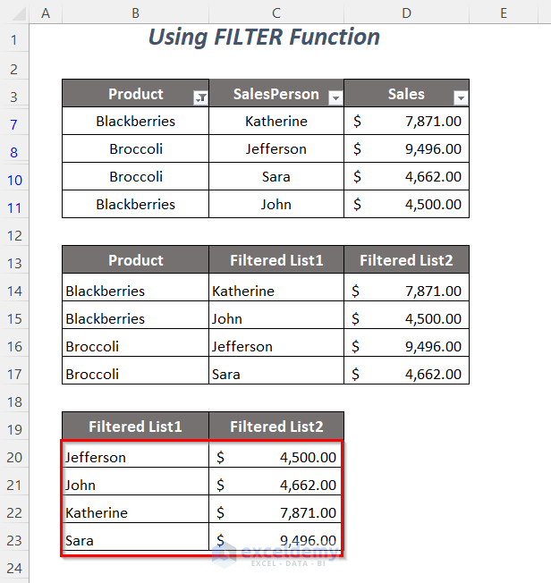
We have copied the filter dropdown list of the Salesperson column to the Filtered List1 column.
The filter dropdown list of the Sales column in the Filtered List2 column.
Method 5 – Using a Combination of SUBTOTAL, INDEX, and MATCH Functions
5.1 Getting the Updated Serial Numbers
Steps:
We will get the serial numbers in the Helper column which will be automatically updated after filtering.
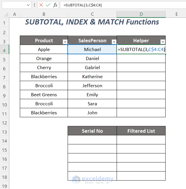
- Enter the following formula in cell D4:
=SUBTOTAL(3,C$4:C4)Here, 3 is for the COUNTA function, and C$4:C4 is the range that will be updated for each successive row. For Row 8, it will be C$4:C8 because we have fixed the first limit by putting a $ sign before Row 4.
- Press ENTER and drag down the Fill Handle tool.
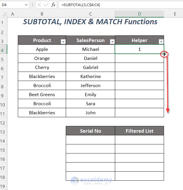
We will get the serial numbers in the Helper column.
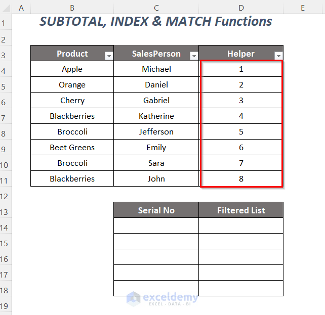
We will filter the table based on the Product column, and so we have checked the products Apple, Beet Greens, Blackberries, and Cherry from the dropdown list of this column.
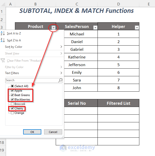
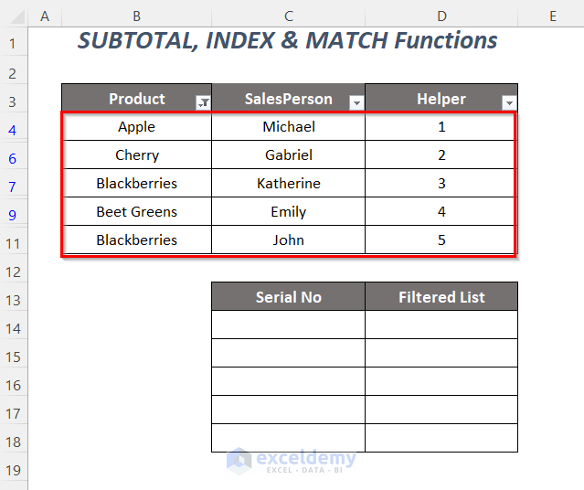
We will get the following filtered table.
- Copy the filter dropdown list of the SalesPerson column to the Filtered List column.
5.2 Using the INDEX and MATCH Functions to Extract the List
Steps:
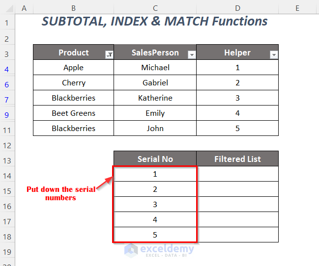
- Enter the serial numbers in the Serial No column.
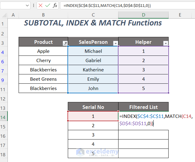
- Enter the following formula in cell D14:
=INDEX($C$4:$C$11,MATCH(C14,$D$4:$D$11,0))Here, $C$4:$C$11 is the range of the SalesPerson column that we want to get, and C14 is the serial number that will be matched with the numbers in the Helper column.
- MATCH(C14,$D$4:$D$11,0) → returns the row index number of the value in cell C14 which is 1.
Output → 1
- INDEX($C$4:$C$11,MATCH(C14,$D$4:$D$11,0)) becomes
INDEX($C$4:$C$11,1) → checks the corresponding value in the range $C$4:$C$11 for row index number 1
Output → Michael
- Press ENTER and drag down the Fill Handle tool.
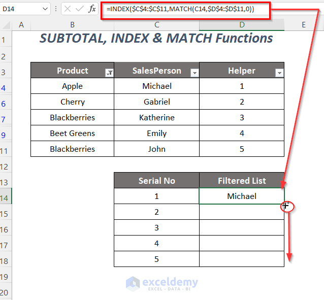
You will get the salespersons’ names in the Filtered List column, and the final task is to sort them from A to Z.
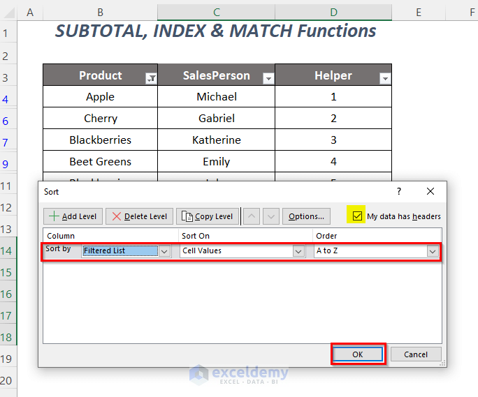
- Select the dataset and go to the Data Tab >> Sort & Filter Group >> Sort Option.

- The Sort dialog box will open up.
- Select the following: Sort by → Filtered List; Sort On → Cell Values; Order → A to Z.
- Click on the My data has headers option and press OK.
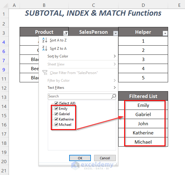
The list will be sorted, and we will get a copy of the filter drop-down list of the SalesPerson column in the Filtered List column.
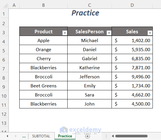
Practice Section
Here is a Practice dataset for you to use.
Download the Practice Workbook
Related Articles
- How to Create a Drop Down List from Another Sheet in Excel
- Create Excel Drop Down List from Table
- How to Remove Drop Down List in Excel
- How to Link a Cell Value with a Drop Down List in Excel
- How to Auto Update Drop-Down List in Excel
- How to Create Excel Drop Down List with Color
- How to Create Drop Down List with Filter in Excel
- How to Add Item to Drop-Down List in Excel
- How to Create a Drop Down List with Unique Values in Excel
- Excel Drop Down List Not Working
<< Go Back to Excel Drop Down List Filter | Excel Drop-Down List | Data Validation in Excel | Learn Excel
Get FREE Advanced Excel Exercises with Solutions!
