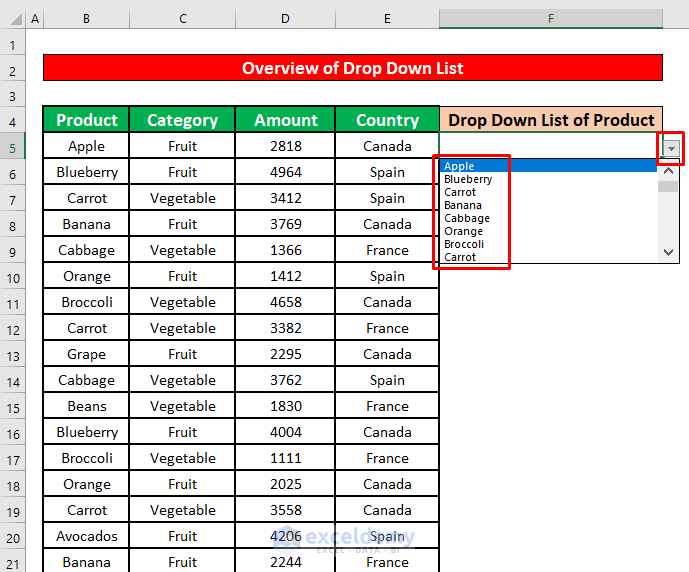
How to Remove Duplicates from a Drop Down List in Excel (4 Methods)

Dataset Overview

Let’s assume you have a large Excel worksheet containing information about various fruits and vegetables imported by a country into three different European countries. The dataset includes columns for Product Name, Product Category, Exported Amount, and Importer Country.

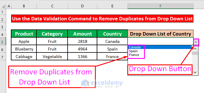
Our goal is to create a drop-down list and remove any duplicate values from it.

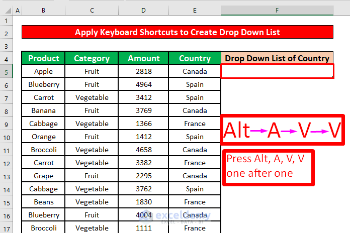
Method 1 – Keyboard Shortcuts

Create a drop-down list from your dataset using the following keyboard shortcuts:
- Press Alt + A + V + V sequentially.
- This opens the Data Validation dialog box.

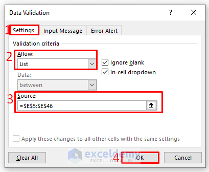
In the Data Validation dialog box:
- Select Settings.
- Choose List from the Allow dropdown.
- Enter the range of your data (e.g., =$E$5:$E$46) in the Source box.
- Click OK.

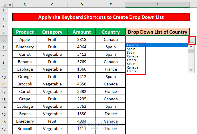
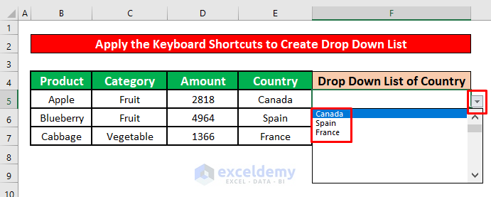
You now have a drop-down list corresponding to the countries, but it may contain duplicate values.

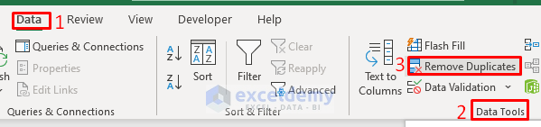
To remove duplicates:
- Go to the Data tab.
- Navigate to Data Tools and select Remove Duplicates.

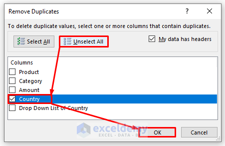
In the Remove Duplicates dialog box:
- Click Unselect All.
- Check the Country option.
- Click OK.

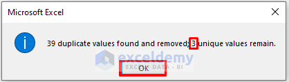
A window will appear, indicating that 39 duplicate values were found and removed, leaving 3 unique values.

Method 2 – Data Validation Command

From the Data tab, go to Data Tools, select Data Validation and click on Data Validation.

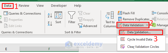
Create a Data Validation dialog box by repeating steps 2 and 3 from Method 1.
The resulting drop-down list will now be free of duplicates.

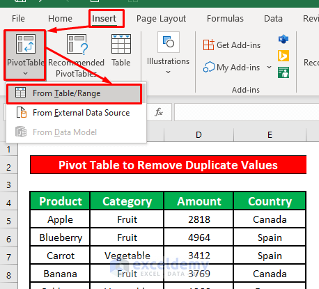
Method 3 – Create a Pivot Table

Go to the Insert ribbon, select Tables, choose PivotTable and select From Table/Range.

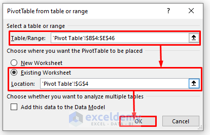
In the PivotTable from table or range dialog box:
- Choose the range of cells for your dataset (e.g., ‘Pivot Table’!$B$4:$B$46).
- Check the Existing Worksheet option.
- Click OK.

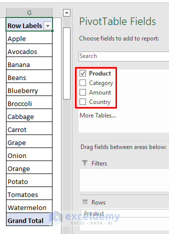
This creates a Pivot Table. Select only the Product option as shown in the screenshot. The Pivot Table automatically removes duplicate values.

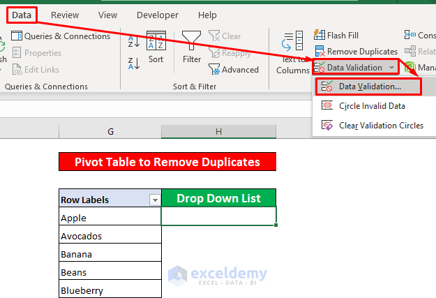
Add a heading named Drop Down List in cell H4 of your data table.
Go to the Data tab, select Data Tools, click on Data Validation and choose Data Validation.

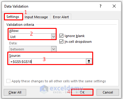
In the Data Validation dialog box:
- Choose Settings.
- Select List from the Allow dropdown.
- Enter the range =$G$5:$G$18 in the Source box.
- Click OK.

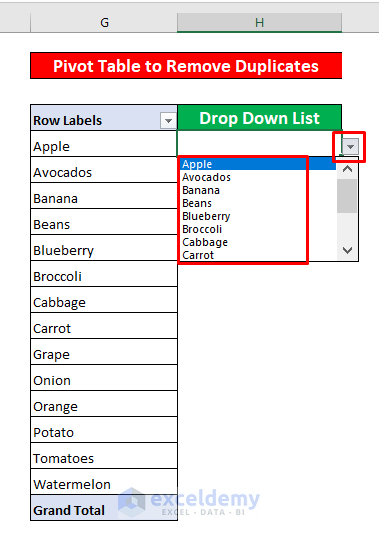
You now have a drop-down list corresponding to the Product Name without any duplicate values.

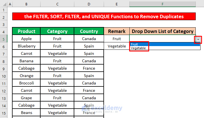
Method 4 – Combine the SORT, FILTER, and UNIQUE Functions

Remove duplicate values from column C (which contains the product categories) using the following formula in cell E5:

=SORT(FILTER(UNIQUE(C5:C46),UNIQUE(C5:C46)<>0))

Formula Breakdown:

The UNIQUE function finds out the unique value from cells C5 to C46.
The FILTER function filters the value from cells C5 to C46 to get a unique value.
The SORT function will sort the data by Category.

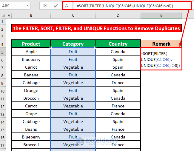
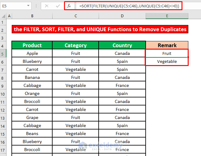
Press ENTER to get the unique product category values.

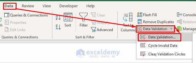
Add a heading named Drop Down List of Category in cell F4 of your data table.
Go to the Data tab, select Data Tools, click on Data Validation and choose Data Validation.

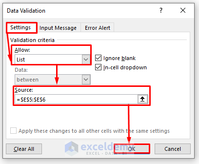
In the Data Validation dialog box:
- Choose Settings.
- Select List from the Allow dropdown.
- Enter the range =$E$5:$E$6 in the Source box.
- Click OK.