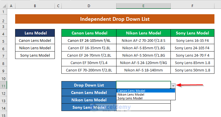
Method 1 – Creating an Independent Drop-Down List
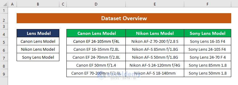
In the dataset below, we see Camera Lens Models and prospective model names. We will use these columns to create drop-down lists.
Steps:
- Create another table anywhere in the worksheet.
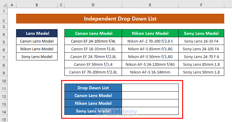
- Create a drop-down list using the above model names.
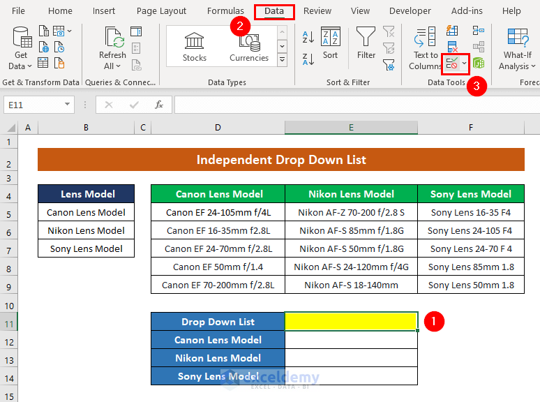
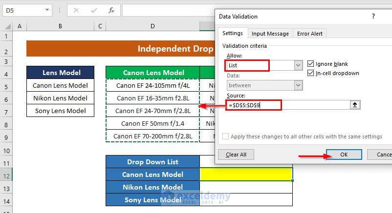
- Select the cell where you want to create a dropdown list (i.e. Cell D11) ->go to the Data tab ->click on Data Validation.
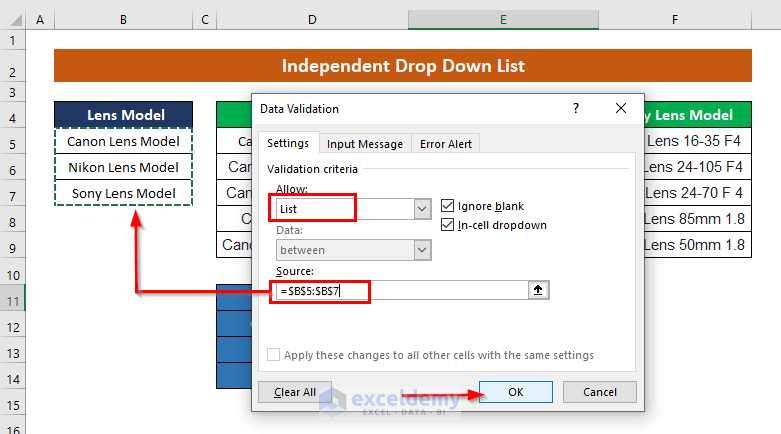
- In the Data Validation dialogue box, select “List”. The Source field window opens. Select the data range from the “Lens Model” column ($B$5:$B$7).
- press OK.
- Click on the icon beside cell D11 to view the list.
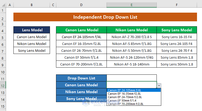
- Create another list beside the cell named “Canon Lens Model” (D12). Repeat the previous procedures and select the data array ($D$5:$D$9) as your source field.
- Press OK to make the list.
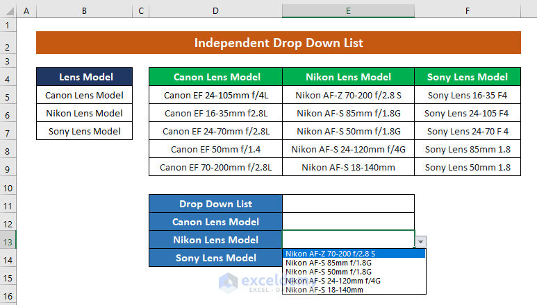
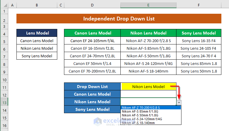
- Create two drop-down lists for two other cells. For the “Nikon Lens Model”, the list is:
- Here, for the “Sony Lens Model”:
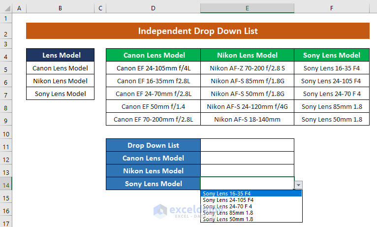
- Choose options from the lists. For example, for the Nikon Lens Model, choose the perspective Lens.
Read More: Create a Searchable Drop-Down List in Excel
Method 2 – Using OFFSET Function in Multiple Columns
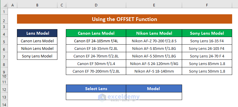
In the below dataset, we have created additional columns containing “Select Lens”, and “Model”.
Steps:
- Create a drop-down list in cell D13 using the data from the “Headers” of the lens model columns. Follow this step like in Method 1.
D13→Data tab→Data Validation
- In the Data Validation dialogue box, select List as the Validation Criteria.
- Select $D$4:$F$4 as your Source data. Remember to check on the “Ignore Blank” and “In-cell Dropdown”.
- Click OK.
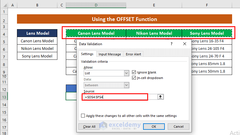
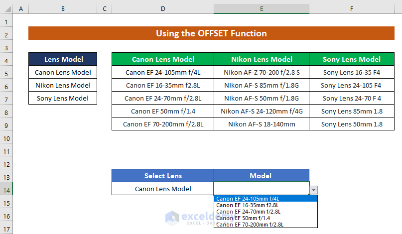
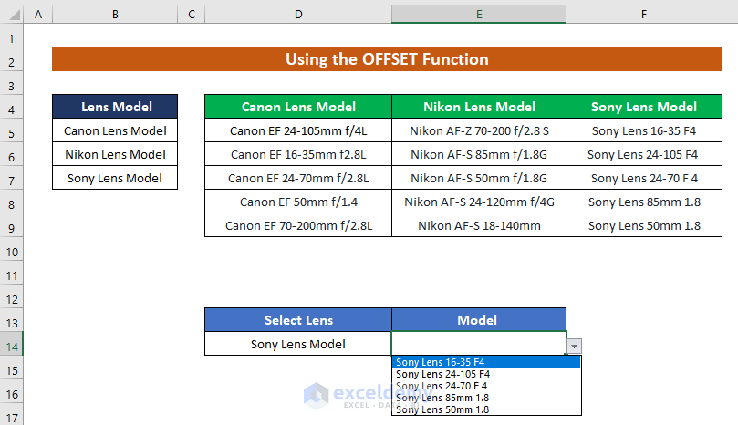
- A drop-down list is created in cell D13. Click on this icon to view the list.
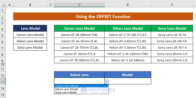
- We will make a final drop-down list using multiple columns.
- Select cell E14 and repeat the process of making the drop-down list as shown in the previous methods.
- In the source box, apply the OFFSET with MATCH functions to use multiple columns simultaneously. The formula is:
=OFFSET($D$4,1,MATCH($D14,$D$4:$F$4,0)-1,5,1)
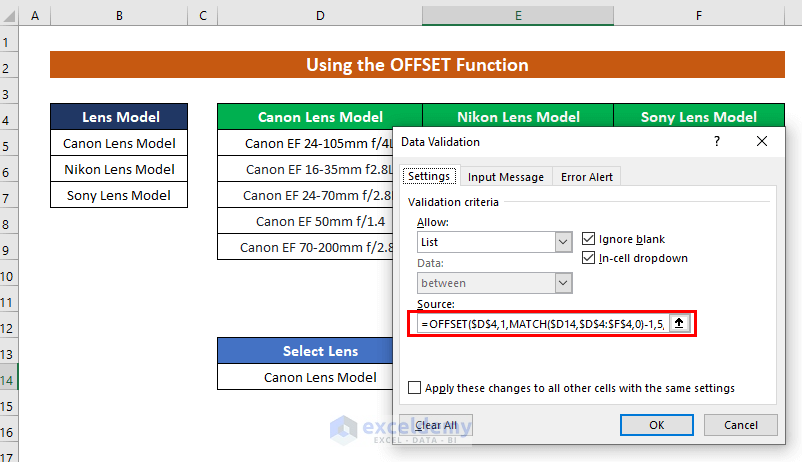
- Reference is $D$4
- The row is 1. We want to move 1 row down each time.
- The column is MATCH($D14,$D$4:$F$4,0)-1. Here, we used the MATCH formula to make the column selection dynamic. In the MATCH formula, the Lookup value is $D14, lookup_array is $D$4:$F$4, and [match_type] is EXACT.
- [height] of each column is 5.
- [width] of each column is 1.
- Click “OK” to get the list from the multiple columns.
Read More: Creating a Drop-Down Filter to Extract Data Based on Selection in Excel
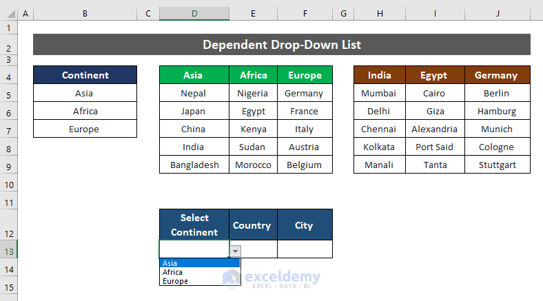
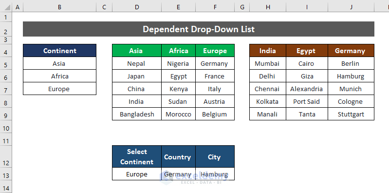
Method 3 – Creating a Dependent Drop-Down List
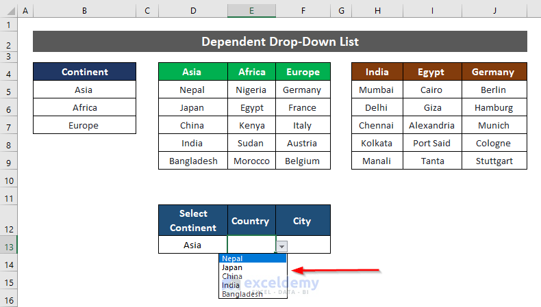
In the dataset below, continents are listed under the column “Continent.” The second set of columns shows country names under their respective continents, and the third shows city names under their respective countries.

Using these columns, we will create drop-down lists. Create another table anywhere in the worksheet.
Steps:
- Create a drop-down list in cell D13 using the name of the continents. To make the list, follow the previous procedures.
- Select the source data $D$4:$F$4.
- Click OK.
- Click on the icon next to cell D13 to show the list.
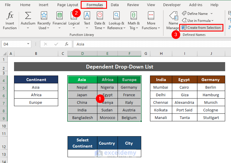
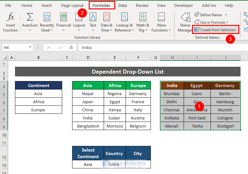
- To create “Name Ranges” for those country columns, select the columns named “Asia”, “Africa”, and “Europe”.
- Go to “Formula” and in the “Name Manager”, click on “Create From Selection”.
Formula → Name Manager → Create from Selection
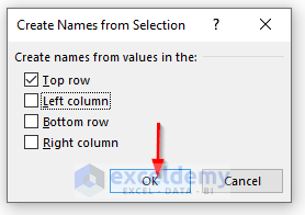
- Check the Top Row and click OK.
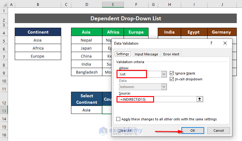
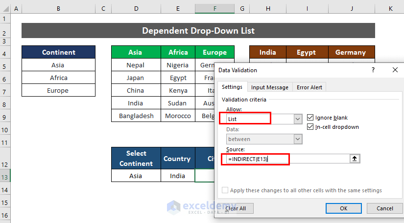
- Select cell E13
- Go to Data Validation and select List. In the Source box, apply the following formula:
=INDIRECT(D13)
When you select Asia in the drop-down list (D13), it refers to the named range “Asia” (through the INDIRECT function and lists all the items in that category).
- Click OK.
- Go to Formulas, and in the Name Manager, click on Create From Selection.
- Check the Top Row and click OK.
- Select cell F13 and go to Data Validation, and select List. In the Source field, apply the following formula:
=INDIRECT(E13)
When you select “India” in the drop-down list (C13), it refers to the named range “India” (through the INDIRECT function) and thus lists all the items in that category.
- Click OK.
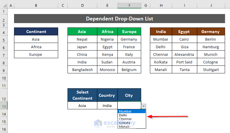
- If you choose “Europe” and the country “Germany,” the list will show us the corresponding results.
Download the Practice Workbook
Download this practice sheet to practice.
Further Readings
- How to Add Blank Option to Drop Down List in Excel
- How to Select from Drop Down and Pull Data from Different Sheet in Excel
- How to Create a Form with Drop Down List in Excel
- How to Remove Used Items from Drop Down List in Excel
- How to Remove Duplicates from Drop Down List in Excel
- How to Fill Drop-Down List Cell in Excel with Color but with No Text
- [Fixed!] Drop Down List Ignore Blank Not Working in Excel
- How to Make Multiple Selection from Drop Down List in Excel
- How to Autocomplete Data Validation Drop Down List in Excel
- Hide or Unhide Columns Based on Drop Down List Selection in Excel
<< Go Back to Excel Drop-Down List | Data Validation in Excel | Learn Excel
Get FREE Advanced Excel Exercises with Solutions!

Very practical and well explained. Thank you
Hello, Nastaran!
Thanks for your appreciation. We are glad that our post helped you.
Regards
ExcelDemy
Hello. Brilliant ideas . I have a remark : at number 3 Idea the data $D$3:$F$3. is wrong you have to write D4:F4 isn’t it ?
Dear Radu,
Thanks for your suggestion and we appreciate it. We updated the cell range.