Dynamic List Excel (Complete Guideline)

In this article, we will show how to create and use a dynamic list in Excel.

We will demonstrate the benefits of using dynamic lists, the formulas and functions used to create them, and the practical applications they provide. Additionally, we will address any limitations or considerations that should be aware of when working with dynamic lists.

You will gain knowledge of useful methods for building dynamic lists, using them to perform operations like data validation, filtering, and sorting, and integrating them with other Excel features like pivot tables and charts.

Download Practice Workbook

Download this practice workbook to exercise while you are reading this article.

What Is a Dynamic List in Excel?

In Excel, a dynamic list is a set of data that automatically changes in size in response to changes in the underlying data. To ensure that any additions, deletions, or modifications in the data source are reflected, it is typically created using Excel formulas or table features.

How to Create Dynamic List Based on Criteria in Excel

1. Using FILTER and OFFSET Functions

Based on Single Criteria:

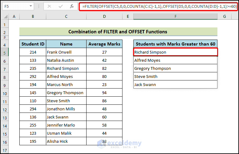
Here we will combine FILTER and OFFSET functions to make a dynamic list of the students whose average marks are greater than or equal to 60.

• Write down the following formula.

Based on Multiple Criteria:

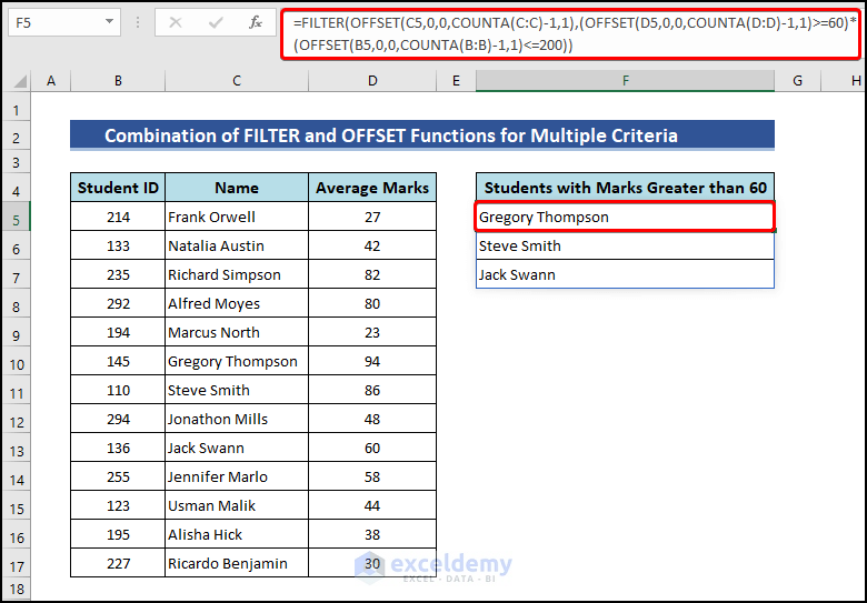
We’ll demonstrate how to make a dynamic list of the students who got marks more than or equal to 60, but whose IDs are less than or equal to 200.

• Write down the following formula.

2. Using INDEX-MATCH with Other Functions

Based on Single Criteria:

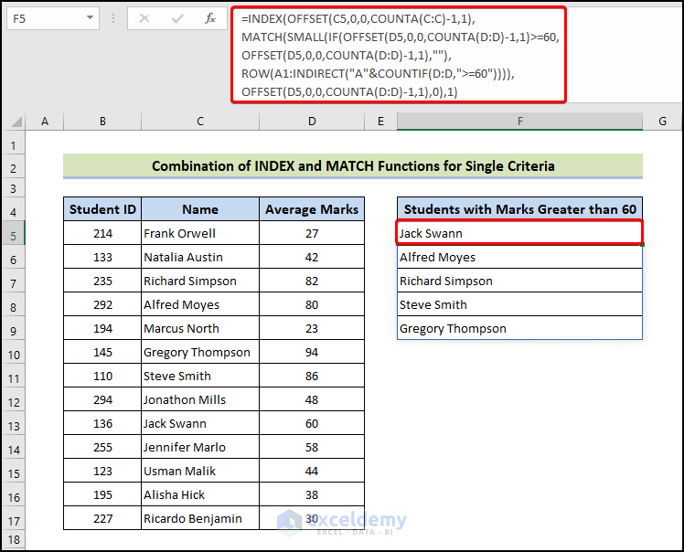
Here we will use Excel’s INDEX-MATCH, OFFSET, SMALL, IF, ROW, COUNTIF, and COUNTIFS functions to create a dynamic list of the students who got more than or equal to 60.

• Write down the following formula.

Based on Multiple Criteria:

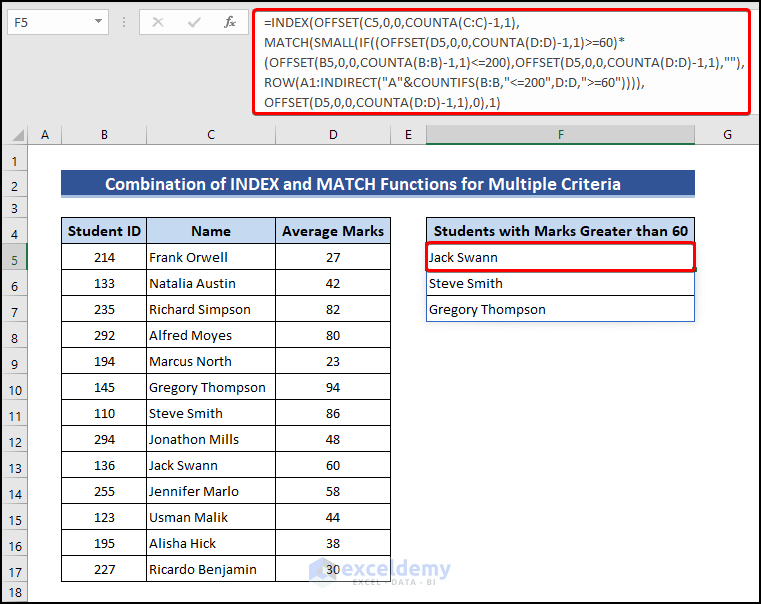
Here we want to get the names of the students who got marks greater than or equal to 60 but have IDs less than 200.

• Write down the following formula.

How to Create a Dynamic Drop-Down List in Excel

Here, we will demonstrate how to create a dynamically generated drop-down list in Excel.

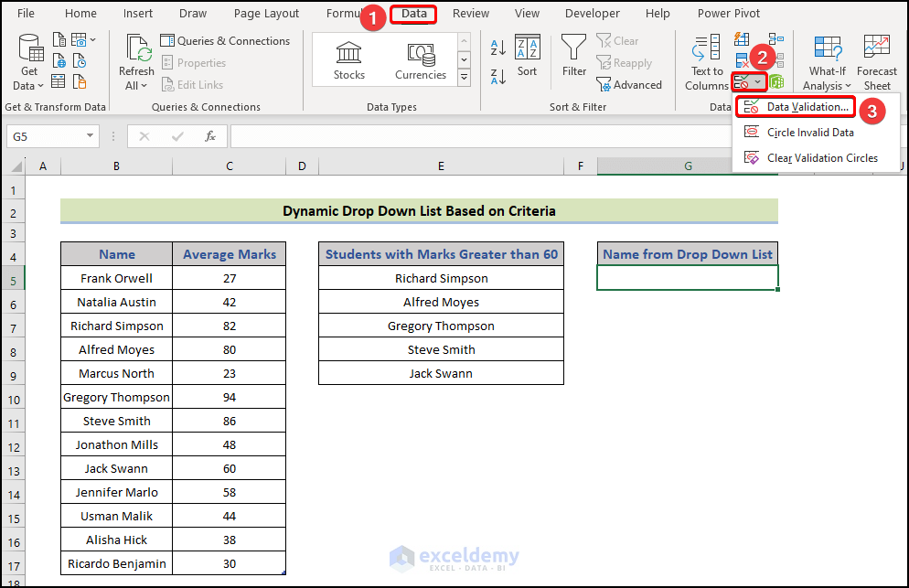
• Select any cell in your worksheet to create the dynamic drop-down list and go to Data > Data Validation > Data Validation under the Data Tools section.

• You will get the Data Validation dialog box. Under the Allow Option, choose List. And under the Source option, enter the reference of the first cell where the list is in your worksheet and a hashtag (#)($E$5# in this example).

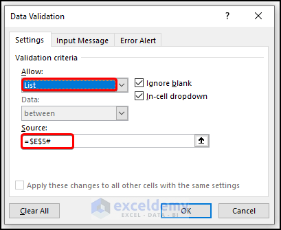
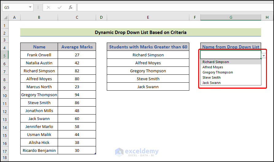
• Then click OK. You will get a drop-down list in your selected cell like this.

How to Create a Dynamic Unique List in Excel

In this section, we will show how to create a unique list by using a combination of UNIQUE and FILTER functions in Excel.

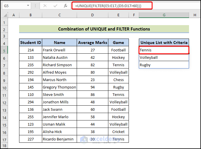
• Write down the following formula.

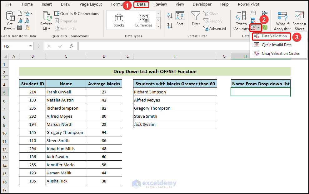
How to Create Dynamic Drop-Down List Using Excel OFFSET

Here, we will demonstrate how to create a dynamically generated drop-down list with the OFFSET function in Excel.

• Select any cell in your worksheet to create the dynamic drop-down list and go to Data > Data Validation > Data Validation under the Data Tools section.

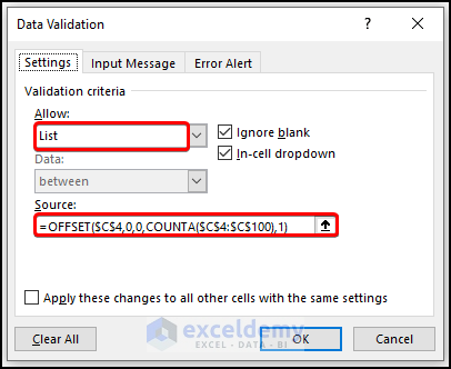
• From the Data Validation dialog box, select List from the drop-down.
• In the source box, write down the following formula.

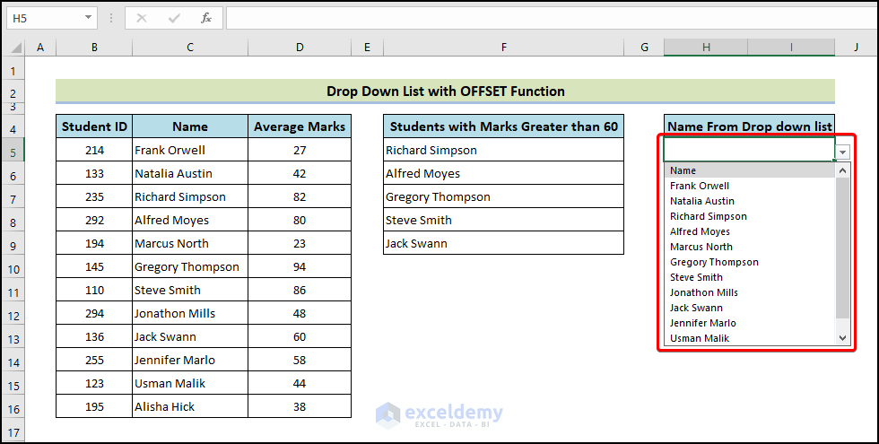
• Then click OK. You will get a drop-down list in your selected cell like this.

Frequently Asked Questions

1. Can I update a dynamic list automatically in Excel?

Yes, a dynamically generated list in Excel updates automatically when the underlying data changes. This ensures that the range expands or shrinks dynamically without manual adjustment.

2. Can I use a dynamic list in combination with other Excel features, such as pivot tables or charts?

Yes, dynamic lists can be combined with other Excel features like pivot tables and charts. By referencing a dynamic list as the data source for these features, they will automatically update as the dynamic list adjusts.

3. Can I use a dynamic list as a source for a dropdown menu in Excel?

Yes, you can use dynamic lists as a source for a dropdown menu in Excel. By setting up data validation with a dynamic list as the source, the dropdown menu will update automatically.

Conclusion

In summary, a dynamic list in Excel is a potent tool that enables the automatic resizing of data ranges in response to modifications in the underlying data.

Excel formulas, tables, or dynamic array functions can be used to create dynamic lists, which can grow or shrink without the need for manual adjustment.

Numerous benefits are provided by doing this, including time savings, automatic updates, and compatibility with other Excel features like data validation, filtering, sorting, pivot tables, and charts.

Dynamic List Excel: Knowledge Hub

• Create Dynamic List in Excel Based on Criteria
• Create Dynamic List From Table
• Create a Dynamic Top 10 List
• Create Dynamic Drop Down List Using Excel OFFSET
• Make Dynamic Drop Down List from Another Sheet
• Create Dynamic Drop Down List Using VBA
• Make a Dynamic Data Validation List Using VBA

<< Go Back to Excel Drop-Down List | Data Validation in Excel | Learn Excel