How to Make a Dynamic Data Validation List Using VBA in Excel

Written by Prantick Bala

Last updated: Dec 14, 2023

In dynamic data validation, when you add a new entry to the source list, the entry is automatically added to the data validation list. It is a very efficient technique to add new data. To make a data validation list dynamic you need to insert a code in Microsoft Visual Basic for Application (VBA). In this article, I’ll show you how you can create a dynamic data validation list in Excel using VBA in 3 easy steps.

Suppose, you have the following dataset where you want to create a data validation list to enter the States name for each Branch Name. You will use the States List in column F as the source list for data validation.

Dynamic Data Validation List Using VBA in Excel: 3 Suitable Steps

1. Create a Dynamic Name Range

First, you have to create a dynamic data validation name range for the States List. To do that,

➤ Go to the Formulas tab and select Name Manager.

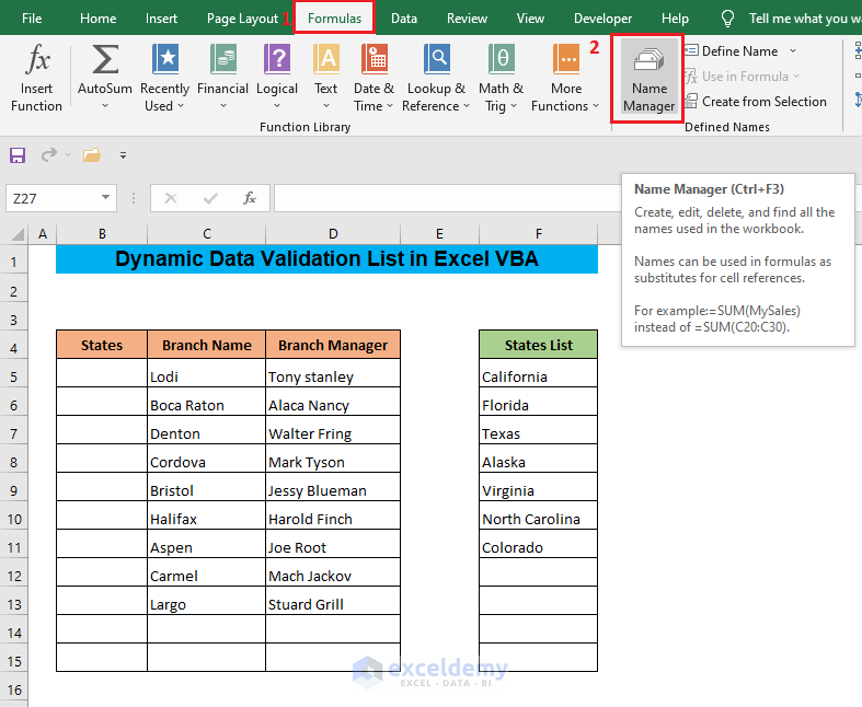
As a result, a Name Manager window will appear.

➤ Click on New in the Name Manager window.

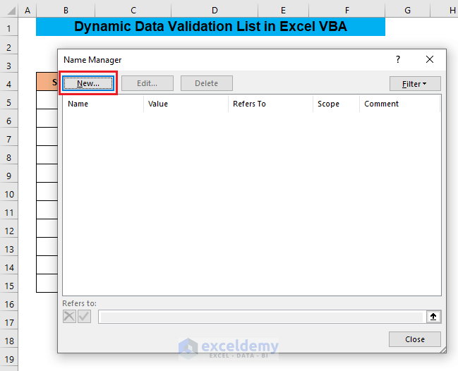
Now, a new window named New Name will appear.

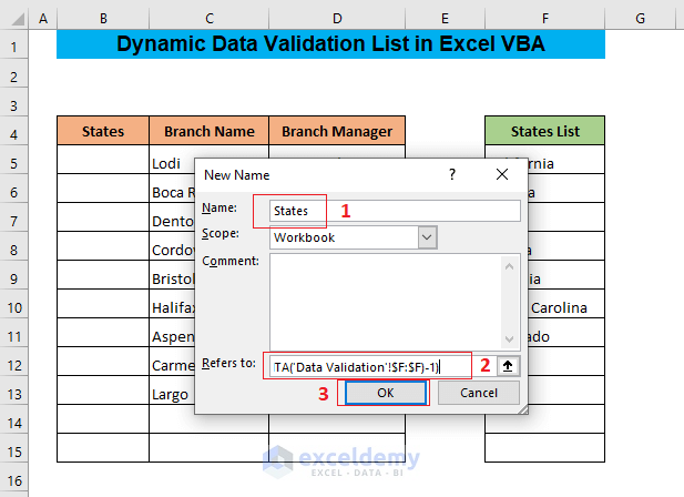
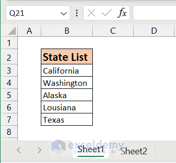
➤ Type a name for the list in the Name box.

For this demonstration, I’ve inserted the name States.

After that,

➤ Insert the following formula in the Refers to box,

=OFFSET('Data Validation'!$F$5,0,0,COUNTA('Data Validation'!$F:$F)-1)

The formula will create a dynamic cell reference for the name States. If you insert any new entry in column F, the name States will be automatically assigned to the entry.

➤ Click on OK.

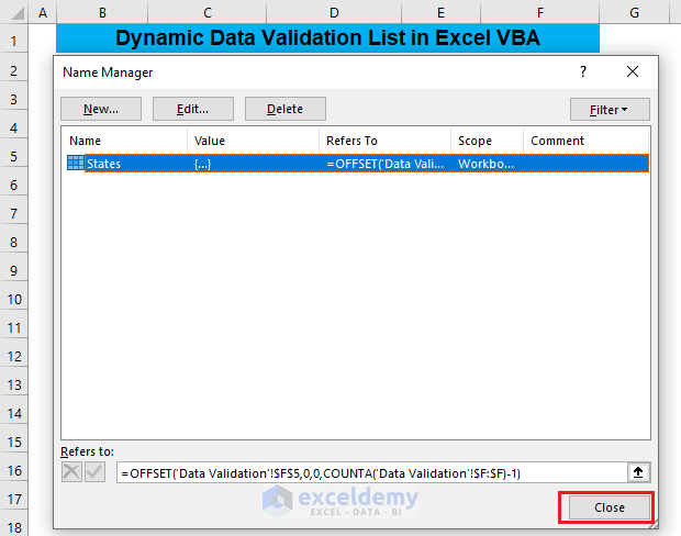
As a result, the name States will be added to the Name Manager.

➤ Click on Close in the Name Manager window.

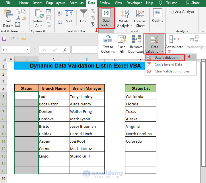
2. Add Data Validation

In this step, you need to add data validation drop down list to the cells of column B. To do that,

➤ Select the cells where you want to add data validation.

➤ Go to Data > Data Tools > Data Validation > Data Validation.

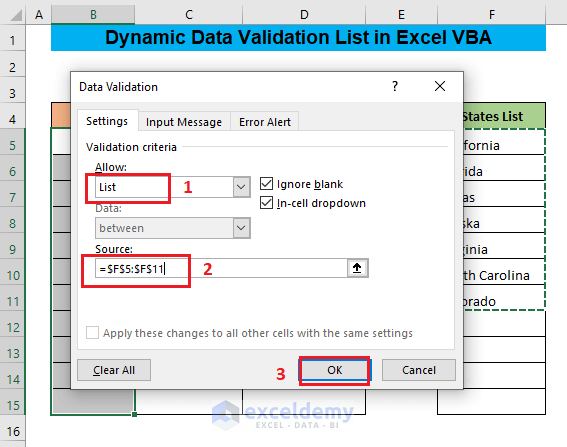
As a result, the Data Validation window will appear. Now,

➤ From the Allow box, select List, and the Source box select the list from column F.

➤ Click on OK.

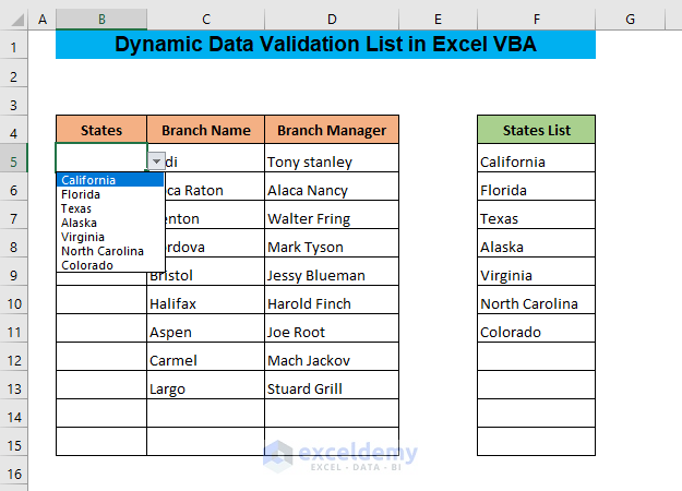
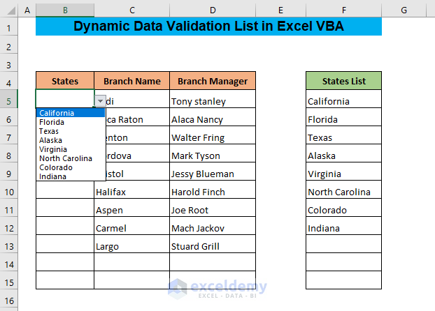
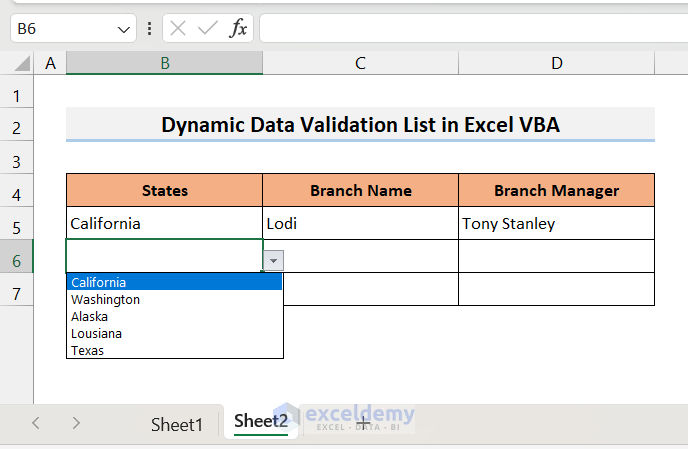
As a result, data validation will be added to the selected cells. Now, if you click on the downward arrow beside the cells of column B a dropdown list will appear. Here, you will see the names of the states of the list of column F.

Now, if you enter a new entry in column F (Here I’ve entered Indiana) and click on the downward arrows beside the cells of column B, you will see that the new entry isn’t showing in the dropdown list.

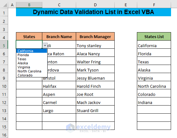
This is happening because your data validation list is not dynamic. To automatically update of new entry you will need to make the list dynamic. You can do that with a simple VBA code which I’ll show you in the next step.

3. Make the Data Validation List Dynamic with VBA

In this section, I’ll add a VBA code to make the validation dynamic. Let’s start the procedure.

➤ Right-click on the sheet name

As a result, a menu will appear.

➤ Select View Code from this menu.

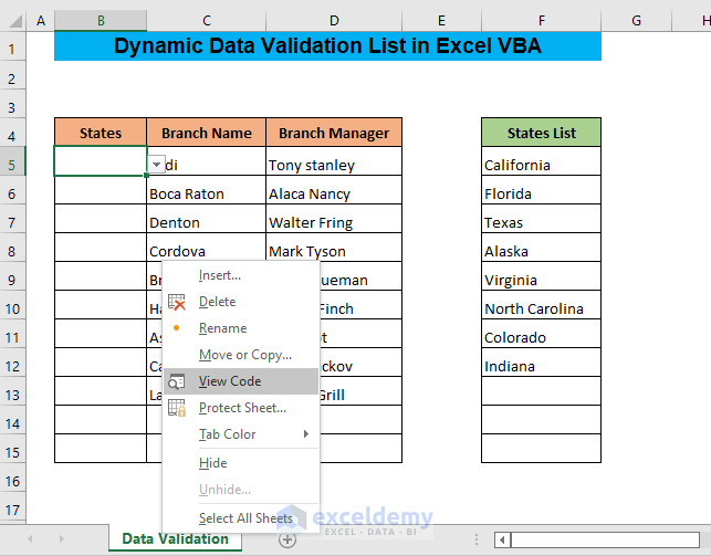
As a result, the Code window of the VBA will be opened.

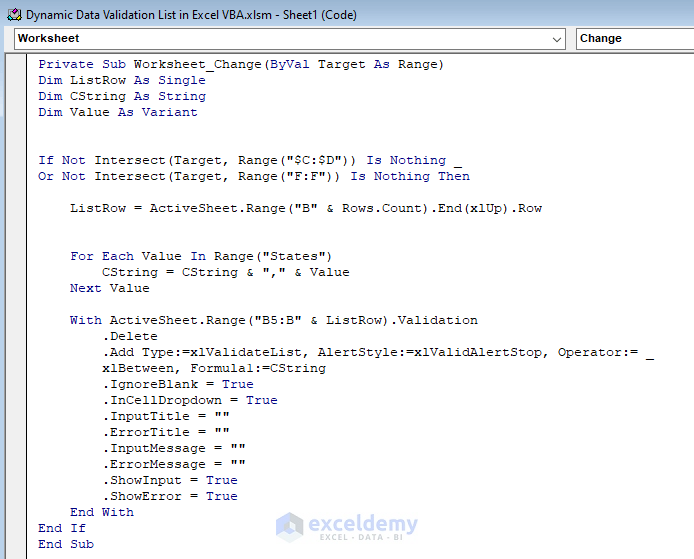
➤ Insert the following code in this window,

Private Sub Worksheet_Change(ByVal Target As Range)

Dim ListRow As Single
Dim CString As String
Dim Value As Variant
If Not Intersect(Target, Range("$C:$D")) Is Nothing _
Or Not Intersect(Target, Range("F:F")) Is Nothing Then
    ListRow = ActiveSheet.Range("B" & Rows.Count).End(xlUp).Row
    For Each Value In Range("States")
        CString = CString & "," & Value
    Next Value
    With ActiveSheet.Range("B5:B" & ListRow).Validation
        .Delete
        .Add Type:=xlValidateList, AlertStyle:=xlValidAlertStop, Operator:= _
        xlBetween, Formula1:=CString
        .IgnoreBlank = True
        .InCellDropdown = True
        .InputTitle = ""
        .ErrorTitle = ""
        .InputMessage = ""
        .ErrorMessage = ""
        .ShowInput = True
        .ShowError = True
    End With
End If

End Sub

The code will change the worksheet in a way that when you insert a new entry in column F, and if there is data in columns C and D of a row, the new entry will be automatically updated in the data validation list of column B of that row.

After inserting the code,

➤ Close the VBA window.

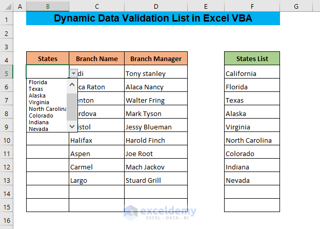
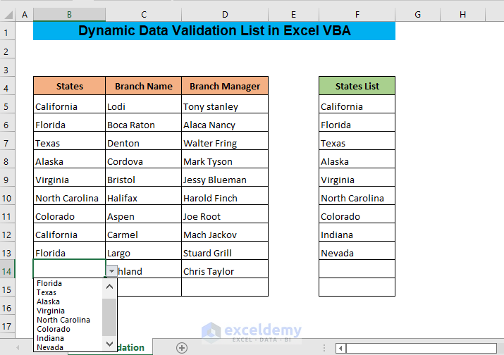
Now, if click on the downward arrows beside the cells of column B, you will see that the new entry Indiana is showing in the dropdown list at this time.

If you add another entry in column F (Nevada), it will be automatically added to the data validation list.

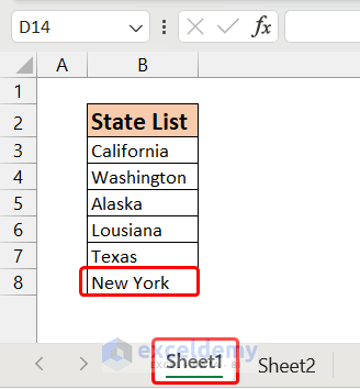
Now, you insert the data from column F in column B by selecting from the dropdown list. If you need to insert new data, you can add that in column F. As a result, the data will automatically appear in the dropdown list. For Example, in cell B15, you need to insert the state name Kentucky which is not listed in column F.

➤ Insert the name Kentucky in column F.

As a result, you will see the name in the dropdown list when you will click on the downward arrow beside cell B15.

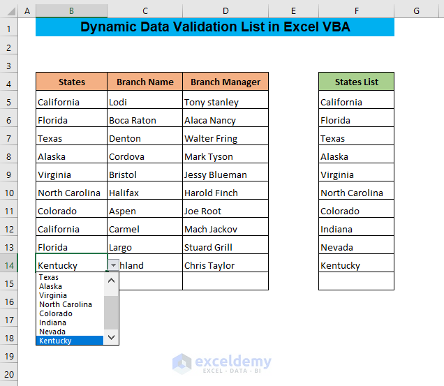
If you want to remove any names from the dropdown list,

➤ Delete the name from column F.

The name will be automatically removed from the dropdown list.

Download Practice Workbook

Dynamic Data Validation List.xlsm

Conclusion

If you don’t insert the VBA code, your data won’t be automatically updated in the dropdown list. The VBA code made the data validation list dynamic. In this article, I’ve discussed how you can create a dynamic data validation list in Excel using VBA. I hope now you’ll be able to create dynamic data validation list according to your needs. If you have any confusion, please feel free to leave a comment.

Get FREE Advanced Excel Exercises with Solutions!

Sub Update_DataValidation() Dim sourceSheet As Worksheet Dim targetSheet As Worksheet Dim sourceRange As Range Dim targetRange As Range Dim lastRow As Long ' Set the source and target sheets Set sourceSheet = Worksheets("Sheet1") ' Change to your source sheet name Set targetSheet = Worksheets("Sheet2") ' Change to your target sheet name ' Find the last row in the source list, assuming the list is in column B lastRow = sourceSheet.Cells(sourceSheet.Rows.Count, "B").End(xlUp).Row ' Define the source range Set sourceRange = sourceSheet.Range("B3:B" & lastRow) ' Assuming data starts from B3 ' Define the target range for data validation, assuming the target range starts at B5 Set targetRange = targetSheet.Range("B5:B" & targetSheet.Cells(targetSheet.Rows.Count, "B").End(xlUp).Row + 1) ' Clear existing data validation in the target range targetRange.Validation.Delete ' Create a dynamic data validation formula Dim formula As String formula = "=" & sourceSheet.Name & "!" & sourceRange.Address ' Apply data validation to the target range With targetRange.Validation .Add Type:=xlValidateList, AlertStyle:=xlValidAlertStop, Operator:= _ xlBetween, Formula1:=formula .IgnoreBlank = True .InCellDropdown = True .ShowInput = True .ShowError = True End With End Sub

9 Comments

Red Apr 26, 2022 at 1:51 AM

im trying to apply this process to a worksheet with multiple sheets:

I have an information template sheet that has my lists for the drop downs and would like to add the drop down to the schedule sheet…

Private Sub Worksheet_Change(ByVal Target As Range)
Dim st As Worksheet
Set st = ThisWorkbook.Sheets(“Schedule Template”)
Dim ListRow As Single
Dim CString As String
Dim Value As Variant
If Not Intersect(Target, st.Range(“$B:$C”)) Is Nothing _
Or Not Intersect(Target, st.Range(“e:e”)) Is Nothing Then
ListRow = st.Range(“B” & Rows.Count).End(xlUp).Row
For Each Value In Range(“ClassLocations”)
CString = CString & “,” & Value
Next Value
With st.Range(“E14:E” & ListRow).Validation
.Delete
.Add Type:=xlValidateList, AlertStyle:=xlValidAlertStop, Operator:= _
xlBetween, Formula1:=CString
.IgnoreBlank = True
.InCellDropdown = True
.InputTitle = “”
.ErrorTitle = “”
.InputMessage = “”
.ErrorMessage = “”
.ShowInput = True
.ShowError = True
End With
End If

End Sub

this is throwing errors
- Reply
  Sabrina Ayon Aug 22, 2022 at 11:57 AM
  
  Hello, Red!
  In the 10th line, there is a correction.
  For Each Value In st.Range(“ClassLocations”)
  Try this!
  And make sure you are writing the code in a Module.
Charles Darwall Jan 15, 2023 at 12:59 AM

Hi there, nice tutorials. But I’m having a devil of a time with it. Using the above download it won’t update the dropdowns in B when I add or remove a State in F. And I am able to add a state in row 15 even if C are empty. I have the latest version of Excel – Office 365
- Reply
  Naimul Hasan Arif Jan 18, 2023 at 11:43 AM
  
  Thank you very much CHARLES DARWALL for your comment. The replies to your 2 problems is mentioned below:
  In my case, the VBA works quite fine. Here, I have Kentucky as the last member in the States List column which is also the last member in the drop-down in cell B13.
  
  Now, I have removed Kentucky as the last value in the States List column. So, Nevada is now the last value in the States List column which is also the last value in the drop-down.
  
  After that, I have added Washington D.C. as the latest last member which has also been updated automatically in cell B12.
  
  On the topic of your second question about being able to add a state in row 15 even if C is empty is because I have selected the range B5:B15 to add the drop-down list with the values in States List.
Charles Darwall Jan 22, 2023 at 12:20 AM

Thanks Naimul (or Arif, apologies), your solution worked perfectly and explanation very clear. Thank you for that.

I have a different question for you regarding the list in column F. What if those names include a comma such as “Doe, John”. My Excel setting (and those of colleagues) reads the comma as a separator. Because of this the drop-down displays Doe and John into sparate selection values. I cannot change Excel settings to use ; as separator.

Here the code snippet from above:

Dim CString As String
…
For Each Value In Range(“States”)
CString = CString & “,” & Value
Next Value

I even tried to force replacement of the comma to make it “Doe; John”, with no joy:

nameText = nameText & Replace(nameText, “;”, “,”) & “,”
Next Value

Thanks so much!!

Charles
- Reply
  Naimul Hasan Arif Jan 23, 2023 at 2:54 PM
  
  Thanks for your appreciation. It means a lot.
  To solve your problem, I will suggest you to change your separator from Control Panel. I hope it’ll solve the separator problem.
Charles Darwall Jan 23, 2023 at 8:43 PM

That would work for me but it won’t work for others – the file is on a sharepoint in a large conpany.

Thanks
Wafee Aug 3, 2023 at 9:25 AM

Hi, What if the code look like if my list is in Sheet1 and the Dropdown is in Sheet2?
- Reply
  Aniruddah Alam Aug 8, 2023 at 3:34 PM
  Thank you, WAFEE for reaching out. If your validation list is in a separate sheet, then you need to modify the code in the following way. Follow the steps below.
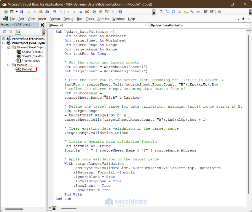
  • First, open a new module and insert the following code in the module.
```
Sub Update_DataValidation()
    Dim sourceSheet As Worksheet
    Dim targetSheet As Worksheet
    Dim sourceRange As Range
    Dim targetRange As Range
    Dim lastRow As Long
    
    ' Set the source and target sheets
    Set sourceSheet = Worksheets("Sheet1") ' Change to your source sheet name
    Set targetSheet = Worksheets("Sheet2") ' Change to your target sheet name
    
    ' Find the last row in the source list, assuming the list is in column B
    lastRow = sourceSheet.Cells(sourceSheet.Rows.Count, "B").End(xlUp).Row
    ' Define the source range
    Set sourceRange = sourceSheet.Range("B3:B" & lastRow) ' Assuming data starts from B3
    
    ' Define the target range for data validation, assuming the target range starts at B5
    Set targetRange = targetSheet.Range("B5:B" & targetSheet.Cells(targetSheet.Rows.Count, "B").End(xlUp).Row + 1)
    
    ' Clear existing data validation in the target range
    targetRange.Validation.Delete
    
    ' Create a dynamic data validation formula
    Dim formula As String
    formula = "=" & sourceSheet.Name & "!" & sourceRange.Address
    
    ' Apply data validation to the target range
    With targetRange.Validation
        .Add Type:=xlValidateList, AlertStyle:=xlValidAlertStop, Operator:= _
        xlBetween, Formula1:=formula
        .IgnoreBlank = True
        .InCellDropdown = True
        .ShowInput = True
        .ShowError = True
    End With
End Sub
```
  • Next, you need to paste the following event driven code in both Sheet1 and Sheet2 modules.
```
Private Sub Worksheet_Change(ByVal Target As Range)
If Not Intersect(Target, Range("$B:$B")) Is Nothing Then
Call Update_DataValidation
End If
End Sub
```
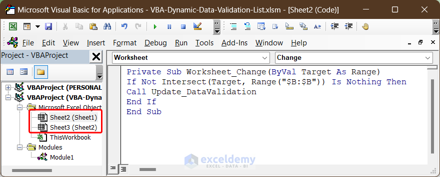
  • The above code will call the Update_DataValidation subroutine whenever you change anything to the B column of the respective sheet. Consequently, the Update_DataValidation subroutine will update the validation options.
  • For example, I have my source list in column B of Sheet1 starting from B3.
  
  • On the other hand, we want to validate column B, starting from cell B5 in Sheet2.
  
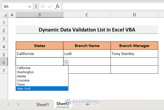
  • Now, I add another state to the source list (for example New York).
  
  5-Adding Value in the Source List
  • As soon as I make change in the list, the Update_DataValidation will run in the background. As a result, I also find New York in the validation list in Sheet2.
  
  6-New Item Added in the Validation List
  
  I hope, the codes and example will be helpful to you.
  
  Regards
  Aniruddah