How to Create Dynamic Drop Down List Using VBA in Excel

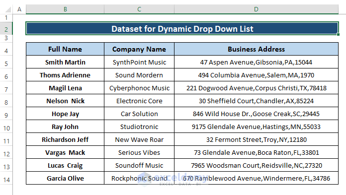
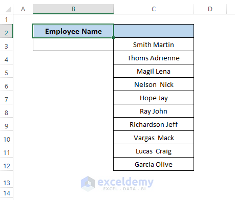
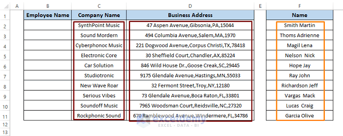
Let’s say we have a dataset where Employee Name, Company Name, and Business Addresses are displayed. We want a dynamic drop-down list where we can assign any employee name besides the Company Name and Business Addresses.

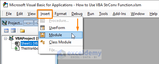
Opening Microsoft Visual Basic and Inserting Code in the Module

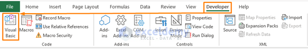
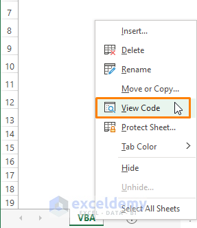
There are mainly 3 ways to open Microsoft Visual Basic window:

• Using Keyboard Shortcuts: Press Alt + F11 to open the Microsoft Visual Basic window.
• Using Developer Tab: In an Excel worksheet, go to Developer Tab and select Visual Basic.

• Using Worksheet Tab: Go to any worksheet, right-click on it, and choose View Code from the Context Menu.

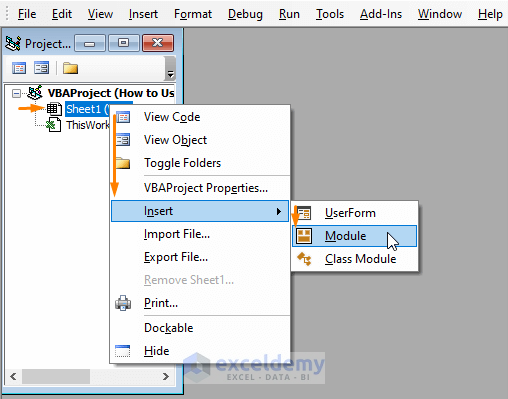
Inserting a Module in Microsoft Visual Basic: There are 2 ways to insert a Module in Microsoft Visual Basic window:

• Select a Worksheet and Right-Click on it, then select Insert (from the Context Menu) and choose Module.

•  Select Insert from the Toolbar and choose Module.

Dynamic Drop-Down List in Excel Using VBA: 2 Easy Ways to Create

Method 1 – Range to Create a Dynamic Drop-Down List in Excel

From the dataset, we know that our worksheet contains multiple employee names. We want to create a dynamic drop-down list using the range (i.e., C column).

Steps:

• Open Microsoft Visual Basic then insert a Module using the instruction section.
• Paste the following macro in any Module:

Sub Dynmc_DropDown_Range()
Dim wrk As Worksheet: Set wrk = Worksheets(2)
Dim nameText As String
Dim nameRng As Range
nameText = "DynamicList"
Set nameRng = wrk.Range("$C:C")
ThisWorkbook.Names.Add Name:=nameText, RefersTo:=nameRng
With Worksheets(2).Cells(3, "B").Validation
.Delete
.Add Type:=xlValidateList, AlertStyle:=xlValidAlertStop, _
Operator:=xlBetween, _
Formula1:="=" & nameRng.Address
End With
End Sub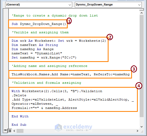

 ➤ in the code,

1 – start the macro procedure by declaring the Sub name. You can assign any name to the code.

2 – declare the variable then assign the variable to create a DynamicList in the Name Manager. Also assign the range (i.e., $C:C).

3 – assigns the names and range to the Worksheet2.

4 – data validation starts from row 3 in column B using the WITH statement and displays the nameRng (i.e., column C) entries in the validation.

• Press F5 to run the macro.
• After returning to the workbook, click on the drop-down icon.
• We see all the entries from column C are present in the drop down list as depicted below picture.

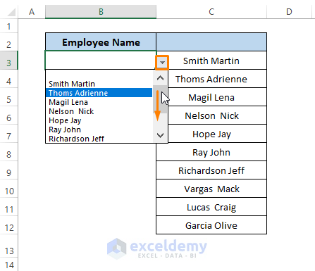
• Add another name (i.e., Jenny Anderson) to the column, then click on the drop-down icon in column B. You find out the last entry is added automatically to the list.

Read More: How to Make a Dynamic Data Validation List Using VBA in Excel

Method 2 – Dynamic Drop-Down List Using Name Manager

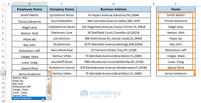
In Method 1, we created only one drop-down dynamic list box. In this method, we’ll create as many drop-down list boxes as the data requires. Our dataset is organized as shown in the below image. We want column F’s Name entries in column B (i.e., Employee Name) to assign the Company and Addresses.

Steps:

• Select the Range (i.e., C:C) to give it a Name.
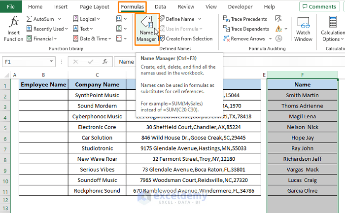
• Go to the Formulas tab and click on Name Manager (from the Defined Names section).

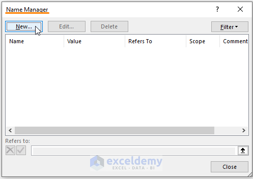
• The Name Manager window opens. Click on New.

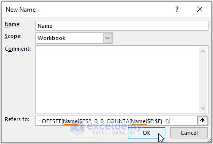
• In the New Name window, type a name in the Name dialog box.
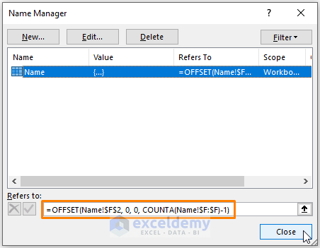
• Paste the below formula in the Refers to command box:

The OFFSET function takes Name!$F$2 as the reference, 0 and 0 as rows and columns. In the end, COUNTA (Name!$F:$F)-1 portion as the range height. 1 is subtracted from the count to ignore the column heading.

• Click on OK.

• Clicking OK assigns the range (C column) to the Name entity. Click on Close.

• Double-click on the Name sheet. The Name sheet’s macro window opens.
• Paste the following code there:

Private Sub Worksheet_Change(ByVal Target As Range)
Dim mrfrow As Single
Dim nameText As String
Dim Value As Variant
If Not Intersect(Target, Range("$C:$D")) Is Nothing _
Or Not Intersect(Target, Range("F:F")) Is Nothing Then
mrfrow = ActiveSheet.Range("C" & Rows.Count).End(xlUp).Row
For Each Value In Range("Name")
nameText = nameText & "," & Value
Next Value
With ActiveSheet.Range("B2:B" & mrfrow).Validation
.Delete
.Add Type:=xlValidateList, AlertStyle:=xlValidAlertStop, Operator:= _
xlBetween, Formula1:=nameText
.IgnoreBlank = True
.InCellDropdown = True
.InputTitle = ""
.ErrorTitle = ""
.InputMessage = ""
.ErrorMessage = ""
.ShowInput = True
.ShowError = True
End With
End If
End Sub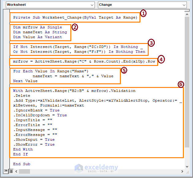

➤ From the above image, in the sections,

1 – begin the macro code declaring the VBA Macro Code’s Sub name.

2 – declare the variables as Single and String and Variant.

3 – impose a condition on targeted ranges using the VBA IF statement. Also, check whether the ranges intersect or not using the VBA Intersect Method.

4 – assign mrfrow to a range (i.e., column C) variable in case of no intersection.

5 – for each value in the range the macro assigns the nameText variable a formula.

6 – VBA With Statement applies data validation in column B ignoring blanks, error messages, etc.

• Return to the worksheet.
• Click on the Drop-Down List icon, where you can see all the names are available to get inserted in column B.

• You can assign all the employee names according to the Name column (i.e., F column) in column B. You can also type a new name, company, and business address in the respective rows, then click on the drop-down list icon.
• After scrolling you see the newly entered name present in the drop-down list.

Read More: How to Use Named Range for Data Validation List with VBA in Excel

Download Excel Workbook

Related Articles

• VBA to Select Value from Drop Down List in Excel
• Excel VBA to Create Data Validation List from Array
• Unique Values in a Drop Down List with VBA in Excel
• Data Validation Drop Down List with VBA in Excel
• How to Make Multiple Dependent Drop Down List with Excel VBA