How to Use Named Range for Data Validation List with VBA in Excel

If you are looking for the easiest ways to use named range for data validation list in Excel VBA, then you will find this article useful. Named ranges are useful to use in a data validation formula to make a dropdown list easily and this task can be made super easy with the help of some VBA codes.
So, let’s start our main article by exploring the ways of using named ranges in a data validation list.

How to Use Named Range for Data Validation List with VBA in Excel: 4 Ways

Here, we have the following dataset containing the records of some products and their respective salesperson’s lists. Using this dataset we will try to show different ways with different VBA codes to use named ranges in a data validation list.

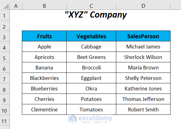
We have used Microsoft Excel 365 version here, you can use any other version according to your convenience.

Method-1: Using Named Range in Data Validation for Making a Dropdown List

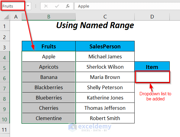
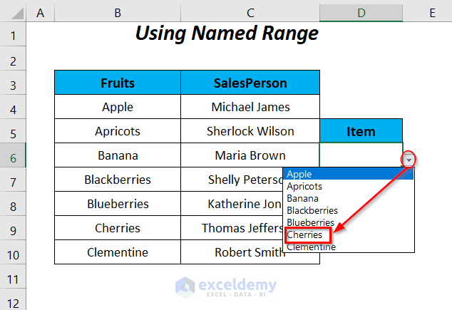
Here, we have named the range of the Fruits column with Fruits and using a VBA code we will create a dropdown list in cell D6.

Step-01:
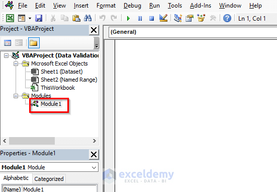
➤ Go to the Developer Tab >> Visual Basic Option.

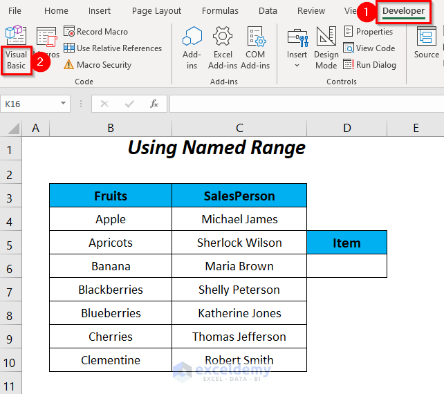
Then, the Visual Basic Editor will open up.
➤ Go to the Insert Tab >> Module Option.

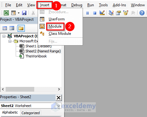
After that, a Module will be created.

Step-02:
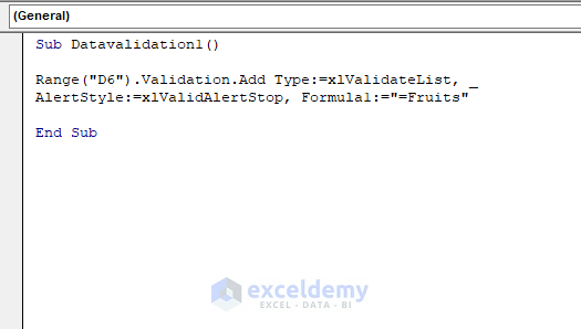
➤ Write the following code

Sub Datavalidation1()

Range("D6").Validation.Add Type:=xlValidateList, _
AlertStyle:=xlValidAlertStop, Formula1:="=Fruits"

End Sub

Here, Validation will be added to cell D6, xlValidateList is for creating a dropdown list and the formula is used as the name of the range “=Fruits”.

➤ Press F5 and later click on the dropdown symbol of cell D6.
Then, you will get the list of the fruits and select any one item from the list like the Cherries.

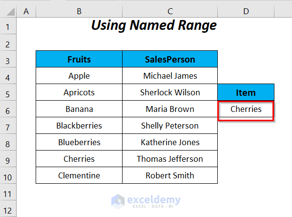
Finally, we are getting our selected item in cell D6.

Read More: Data Validation Drop Down List with VBA in Excel

Method-2: Adding Named Range and a Data Validation List with a VBA Code

We will not create any named range here manually, rather a simple VBA code will form a named range, and then, using it we will get the dropdown list finally in cell D6.

Steps:
➤ Follow Step-01 of Method-1.
➤ Write the following code

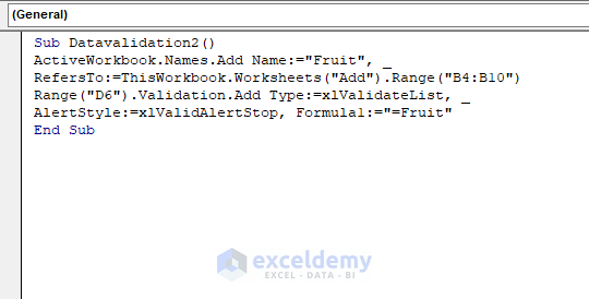
Sub Datavalidation2()

ActiveWorkbook.Names.Add Name:="Fruit", _
RefersTo:=ThisWorkbook.Worksheets("Add").Range("B4:B10")
Range("D6").Validation.Add Type:=xlValidateList, _
AlertStyle:=xlValidAlertStop, Formula1:="=Fruit"

End Sub

Firstly, it will add the name Fruit to the range “B4:B10” of the worksheet Add.
Then, we will add Validation to the cell D6, xlValidateList is for creating a dropdown list and the formula is used as the name of the range “=Fruit”.

➤ Press F5, then, go to the worksheet and click on the dropdown symbol of cell D6.
Later, you will get the list of the fruits and select any one item from the list like the Blueberries.

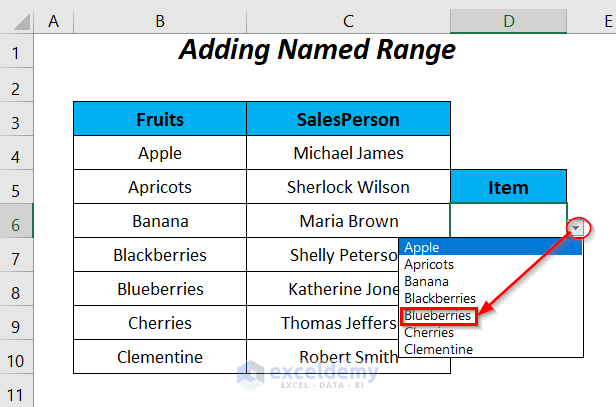
So, we have got our desired item Blueberries from the list and besides this, we can see our created named range for the fruits.

Method-3: Updating Data Validation List with Named Range Using Excel VBA

Suppose, we have the following dropdown list in cell D6, which works fine for the fixed dataset.

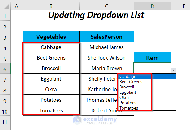
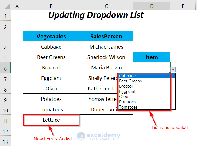
But, if we add an extra vegetable Lettuce then it will not appear in the dropdown list which means our dropdown list is not updated automatically in this case.

To update the list quickly and automatically you can follow this method.

Read More: How to Create Dynamic Drop Down List Using VBA in Excel

3.1: Creating the Updated Named Range

Firstly, we have to add a name for the range of Column B in a way that it will automatically take the newly added items into this name.
➤ Go to the Formulas Tab >> Defined Names Group >> Name Manager Option.

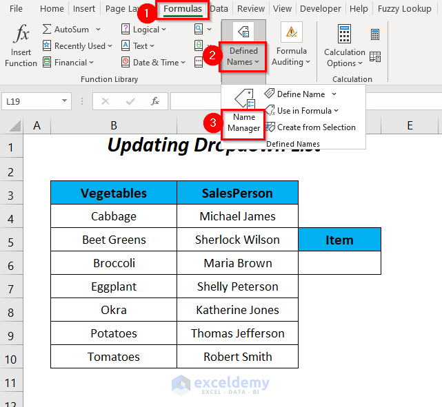
Then, the Name Manager dialog box will open up.
➤ Click on the New option.

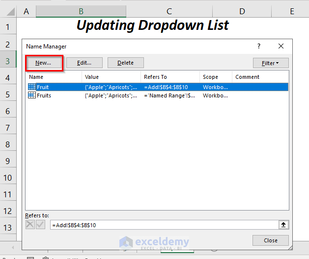
After that, the Edit Name wizard will pop up.
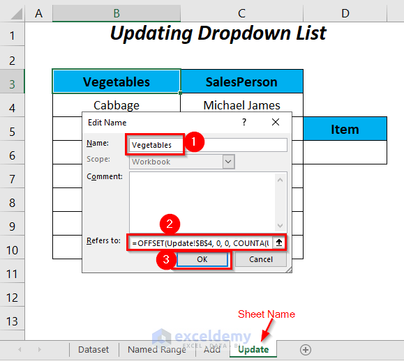
➤ Write down Vegetables in the Name box and the following formula in the Refers to box and finally press OK.

Here, Update! Is the sheet name, $B$4 is the reference cell from which we want to move, 0 for Rows and Columns arguments means it will remain in its reference or starting position.
COUNTA will count the number of cells with any type of values in Column B and then 2 will be subtracted because of the heading of the dataset in B1 and the header of the column in B3. So, you will get only the number of cells containing any vegetables.
This number will be the return reference from the starting position and OFFSET will always return the updated named range here.

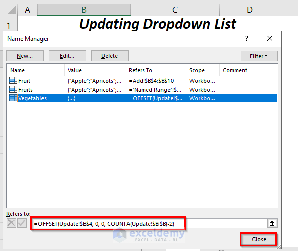
Then, you will be taken to the Name Manager wizard.
➤ Press Close.

3.2: Using a VBA Code to Apply Data Validation List

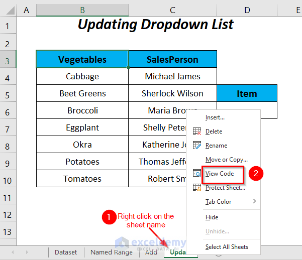
➤ Right-click on the sheet name and select the View Code option.

Afterward, the code window will appear.

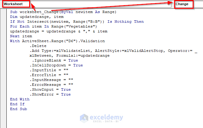
➤ Type the following code

Sub worksheet_Change(ByVal newitem As Range)

Dim updatedrange, item
If Not Intersect(newitem, Range("B:B")) Is Nothing Then
For Each item In Range("Vegetables")
updatedrange = updatedrange & "," & item
Next item
With ActiveSheet.Range("D6").Validation
      .Delete
      .Add Type:=xlValidateList, AlertStyle:=xlValidAlertStop, Operator:= _
       xlBetween, Formula1:=updatedrange
      .IgnoreBlank = True
      .InCellDropdown = True
      .InputTitle = ""
      .ErrorTitle = ""
      .InputMessage = ""
      .ErrorMessage = ""
      .ShowInput = True
      .ShowError = True
End With
End If

End Sub

This code will execute only if any change of values or addition occurred and so we have defined the procedure as Worksheet_Change, Worksheet is the Object and Change is the Procedure.
The newitem contains the address of the cell in which we are adding the new values and we defined it as Range. The data type of updatedrange and item would be considered as Variant, where we have assigned updatedrange to the updated named range of the vegetables and the item is for the values of each cell of this range.
The FOR loop will assign the updated range to updatedrange and the WITH statement will avoid the repetition of the same object, and finally, we have added the validation.

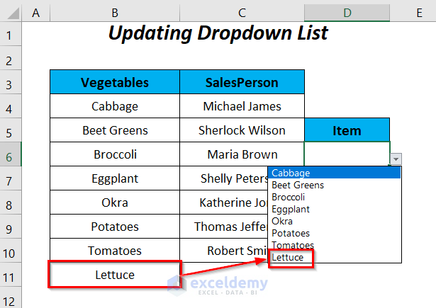
Now, it’s time to return to the main sheet and check out the effect after the addition of a product Lettuce.
As we can see, we have this new item now in our dropdown list.

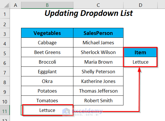
After selecting this new item we are having it in cell D6.

Read More: VBA to Select Value from Drop Down List in Excel

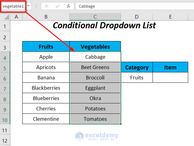
Method-4: Using Named Range for Creating a Conditional Drop Down List

Here, we will create a dropdown list in cell E6 which will be dependent on the condition of cell D6 and for this reason, we have the following two named ranges, such as fruit1 and vegetable1.

Steps:
➤ Follow Step-01 of Method-1.
➤ Write the following code

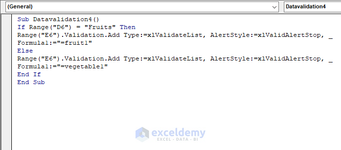
Sub Datavalidation4()

If Range("D6") = "Fruits" Then
Range("E6").Validation.Add Type:=xlValidateList, AlertStyle:=xlValidAlertStop, _
Formula1:="=fruit1"
Else
Range("E6").Validation.Add Type:=xlValidateList, AlertStyle:=xlValidAlertStop, _
Formula1:="=vegetable1"
End If

End Sub

IF-THEN statement will check if the value in cell D6 is Fruits and for this value, as a list, we will get the named range fruit1 as a list in cell E6 otherwise we will get the named range vegetable1 as a list in cell E6.

➤ Press F5, then go to the worksheet and click on the dropdown symbol of cell E6.
After that, you will get the list of the fruits for the category as Fruits in cell D6 and select any one item from the list like the Blackberries.

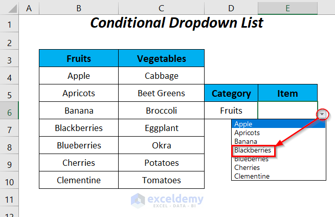
So, we have got our desired item Blackberries from the list.

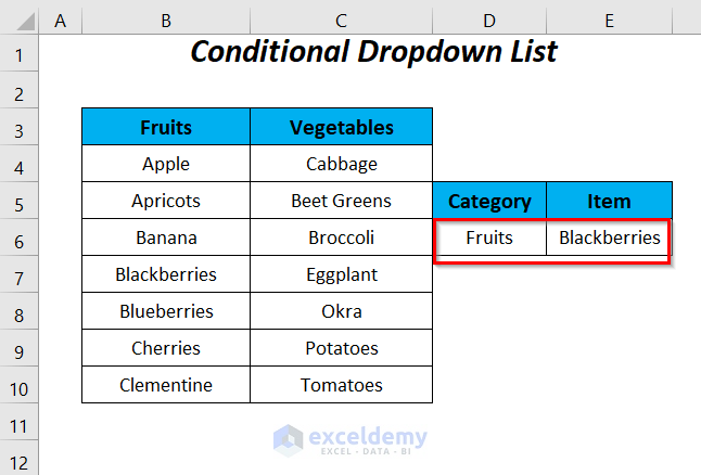
➤ For changing the category as Vegetables we can see that we are having the list of vegetables after running the code.

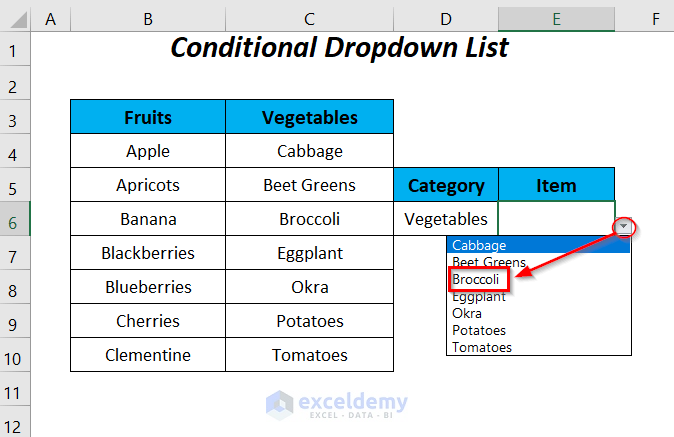
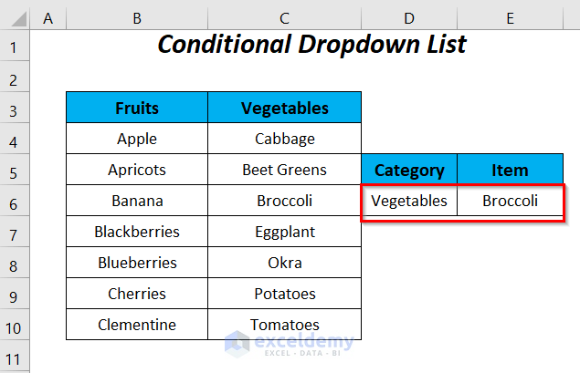
After selecting Broccoli we are getting this item in cell E6.

Practice Section

For doing practice by yourself we have provided a Practice section like below in a sheet named Practice. Please do it by yourself.

Download Workbook

Conclusion

In this article, we tried to cover the ways to use a named range for the data validation list in Excel VBA easily. Hope you will find it useful. If you have any suggestions or questions, feel free to share them in the comment section.

Related Articles

• Excel VBA to Create Data Validation List from Array
• Default Value in Data Validation List with Excel VBA
• Unique Values in a Drop Down List with VBA in Excel
• How to Make a Dynamic Data Validation List Using VBA in Excel
• How to Make Multiple Dependent Drop Down List with Excel VBA