Watch Video – Create a Dynamic Top 10 List in Excel
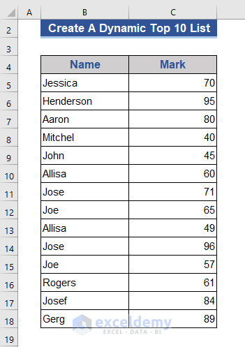
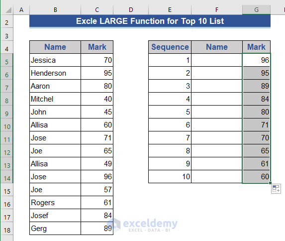
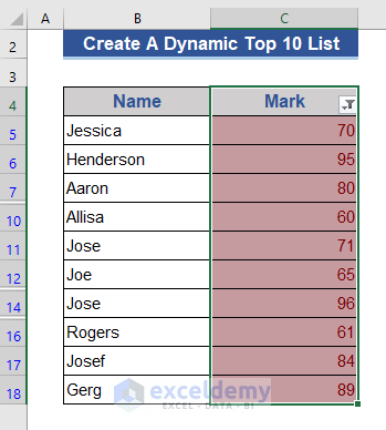
In this article, we’ll discuss several methods to create Dynamic Top 10 lists in Excel. To illustrate our methods, we’ll use the following dataset containing the marks of some students:
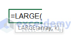
Method 1 – Using LARGE Function
The LARGE function finds the k-th largest number from a given range.
We set 1-10 sequence numbers on the dataset below.
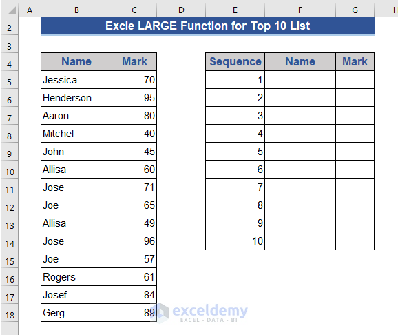
Our process is to calculate the top 10 marks, and then return the corresponding students’ names, using a combination of LARGE and ROW functions.
Steps:
- Go to Cell G5 and enter the formula below:
=LARGE($C$5:$C$18,ROW(F5)-ROW($F$4))
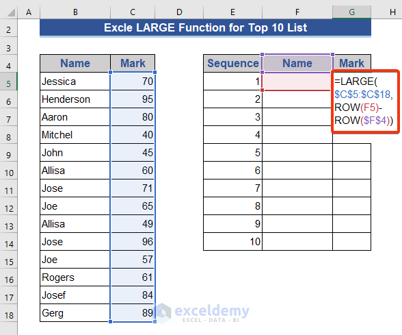
- Press Enter and drag the Fill Handle icon down to Autofill the other cells in the column.
We get the top 10 marks. We can also use the ROWS function for this purpose.
Alternative Formula:
Steps:
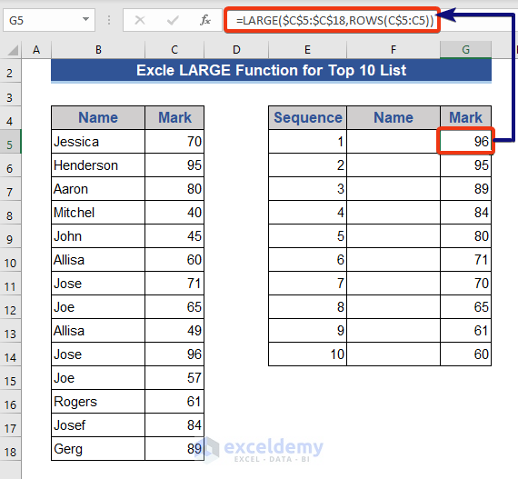
- Enter the following formula in Cell G5:
=LARGE($C$5:$C$18,ROWS(C$5:C5))
- Press Enter and drag the Fill Handle down to fill the rest of the cells.
Now, to show the corresponding names of the top 10 list:
- Go to Cell F5 and enter the following formula:
=INDEX($B$5:$B$18,MATCH(G5,$C$5:$C$18,0))
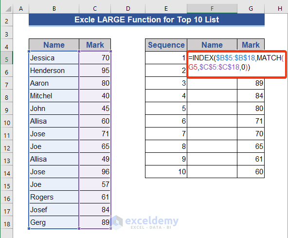
- Press Enter and pull the Fill Handle icon down over the rest of the cells.
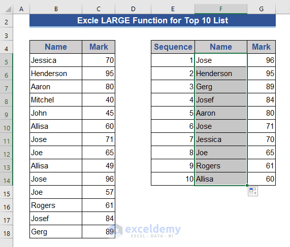
The top 10 names with their marks are returned.
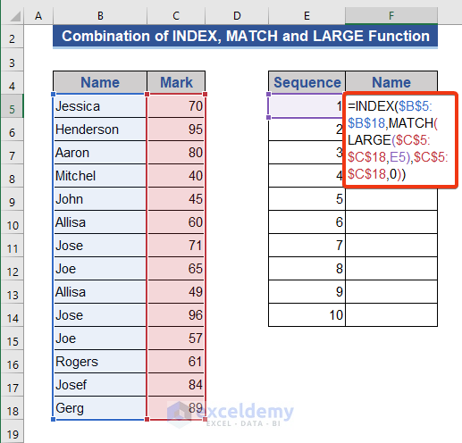
Method 2 – Combining INDEX, MATCH, and LARGE Functions
This method will return the top 10 names directly.
Steps:
- Go to Cell F5 and enter the following formula:
=INDEX($B$5:$B$18,MATCH(LARGE($C$5:$C$18,E5),$C$5:$C$18,0))
- Press Enter and pull the Fill handle icon down.
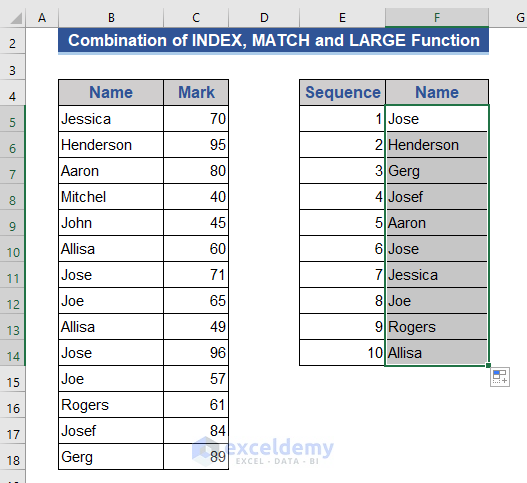
We directly get the top 10 names without the need for another column.
Formula Breakdown:
- LARGE($C$5:$C$18,E5)
This produces the largest number from the range based on the value of Cell E5.
Result: 96
- MATCH(LARGE($C$5:$C$18,E5),$C$5:$C$18,0)
This represents how many results will be shown.
Result: 10
- INDEX($B$5:$B$18,MATCH(LARGE($C$5:$C$18,E5),$C$5:$C$18,0))
This returns the top 10 results from the range.
Result: {Jose, Henderson, Gerg, Josef, Aaron, Jose, Jessica, Joe, Rogers, Allisa}
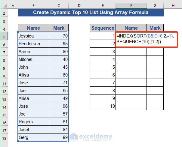
Method 3 – Using an Array Formula
Both the top 10 names and marks of students will show after applying this formula, which is a combination of INDEX, SORT, and SEQUENCE functions.
Steps:
- Go to Cell F5 and enter the formula below:
=INDEX(SORT(B5:C18,2,-1),SEQUENCE(10),{1,2})
- Press Enter and drag the Fill Handle icon.
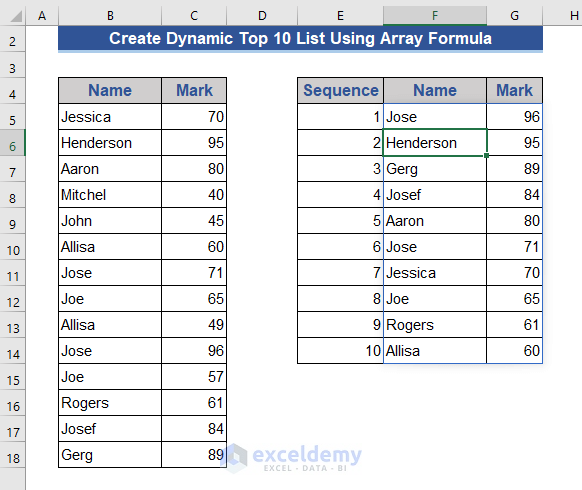
We get both the name and marks simply by applying the formula. No need to drag the formula to copy it.
Formula Breakdown:
- SEQUENCE(10)
Gives a sequence of numbers of 1 to 10.
Result: {1,2,3,4,5,6,7,8,9,10}
- SORT(B5:C18,2,-1)
Sorts the data based on the second column.
Result: {Jose 96, Henderson 95, Gerg 89, Josef 84, Aaron 80, Jose 71, Jessica 70, Joe 65, Rogers 61, Allisa 60, Joe 57, Allisa 49, John 45, Mitchel 40}
- INDEX(SORT(B5:C18,2,-1),SEQUENCE(10),{1,2})
Gives the top ten sorted list.
Result: {Jose 96, Henderson 95, Gerg 89, Josef 84, Aaron 80, Jose 71, Jessica 70, Joe 65, Rogers 61, Allisa 60}
Read More: How to Create Dynamic Drop-Down List Using Excel OFFSET
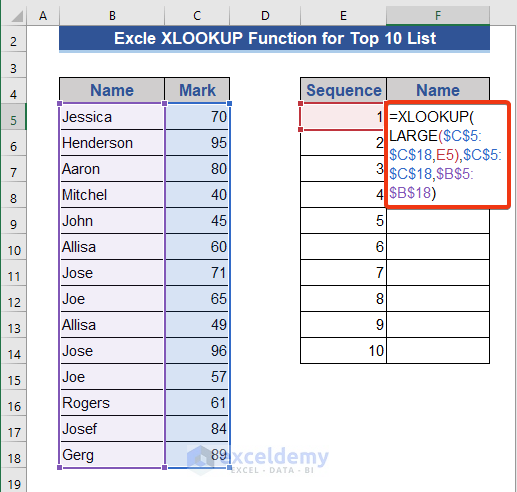
Method 4 – Using XLOOKUP Function
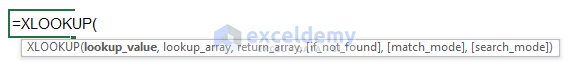
The XLOOKUP function searches objects from a given range or array and return output based on matches.
We will use a combination of the XLOOKUP and LARGE functions here.
Steps:
- Go to Cell F5 and enter the following formula:
=XLOOKUP(LARGE($C$5:$C$18,E5),$C$5:$C$18,$B$5:$B$18)
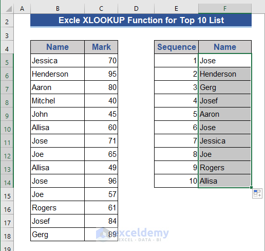
- Press Enter.
- Pull the Fill Handle icon.
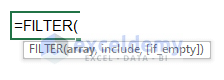
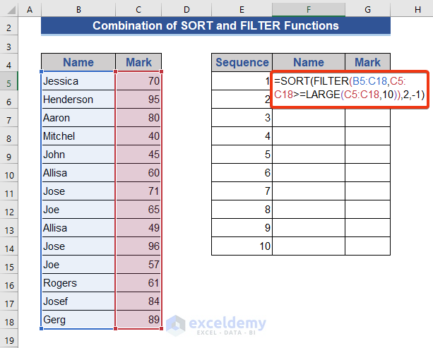
Method 5 – Combining SORT and FILTER Functions
The FILTER function allows filtering a range of values by given criteria.
We will combine the SORT and FILTER functions with the LARGE function here.
Steps:
- Go to Cell F5 and enter the following formula:
=SORT(FILTER(B5:C18,C5:C18>=LARGE(C5:C18,10)),2,-1)
- Press Enter.
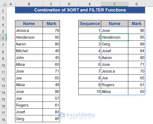
Both the name and mark of students are returned.
Read More: How to Create Dynamic List in Excel Based on Criteria
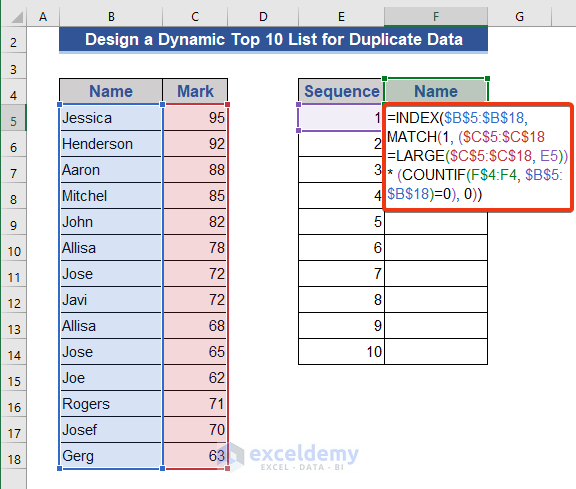
Method 6 – Design a Dynamic Top 10 List for Duplicate Data
This method is suitable for when we have duplicate data.
Steps:
- Go to Cell F5 and enter the formula below:
=INDEX($B$5:$B$18, MATCH(1, ($C$5:$C$18=LARGE($C$5:$C$18, E5)) * (COUNTIF(F$4:F4, $B$5:$B$18)=0), 0))
- Press Enter.
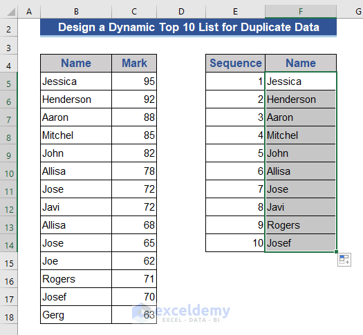
Only the names of students are returned here.
Method 7 – Using Conditional Formatting, Filter, and Sort Tools
Steps:
- Select Cells C5 to C18.
- Click Conditional Formatting from the ribbon.
- Select Top 10 Items from the Top/Bottom Rules.
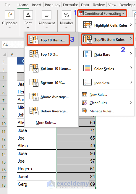
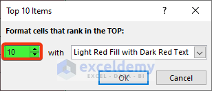
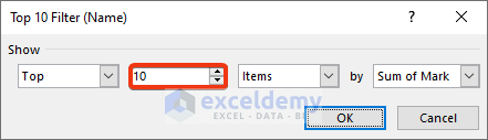
A dialog box will appear. Notice 10, because of the top 10.
- Press OK.
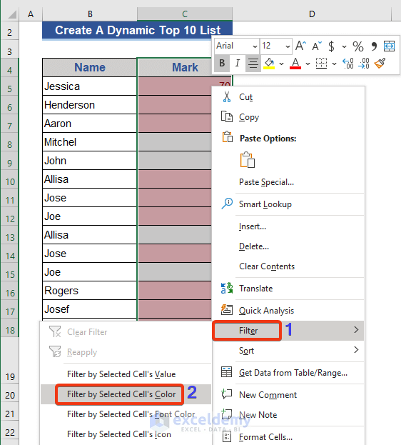
- Select Cells C4 to C18.
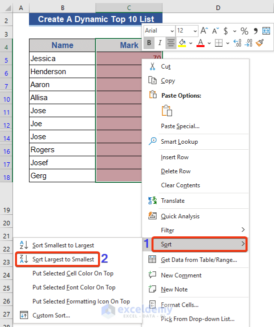
- Click the right button of the mouse.
- Select Filter by Selected Cell’s Color from the Filterlist.
- Click the Filter by Color option.
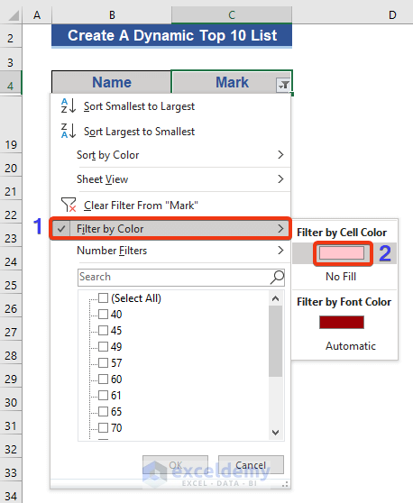
The top 10 data are returned. Now we sort them.
- Click the right button of the mouse.
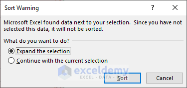
- Select Sort Largest to Smallest from the Sort list.
- Select Expand the selection.
- Click Sort.
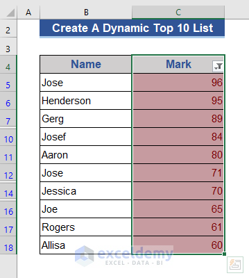
Our top 10 data will be sorted.
Read More: How to Create Dynamic List From Table in Excel
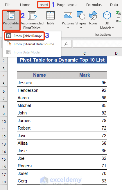
Method 8 – Using Pivot Table
Step 1:
- Go to the Insert tab.
- Select From Table/Range from the PivotTable list.
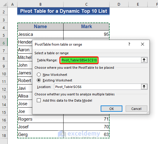
- Select our range from the dataset.
- Press OK.
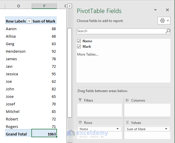
- Tick Name and Mark in the PivotTable Fields.
- Go to Row Labels.
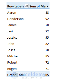
- Select Top 10 from the Value Filters.
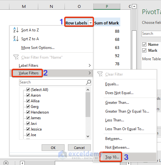
A dialog box will appear.
- Click OK on that box.
Our top 10 list appears, but the data is unsorted.
Read More: How to Make Dynamic Drop Down List from Another Sheet in Excel
<< Go Back to Dynamic List Excel | Excel Drop-Down List | Data Validation in Excel | Learn Excel
Get FREE Advanced Excel Exercises with Solutions!

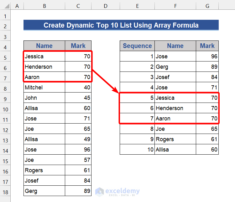
Your article was very useful. But in the case of 2 or 3 persons had the same mark. How could you sort in the list? Thank for your time.
Thank you for your query, DUONG. The third, fifth, and seventh approaches mentioned above can be used safely when numerous people share the same mark. However, their rankings on the Top 10 list are based on where they actually stand on the unsorted list. For instance, Jessica, Henderson, and Aaron will be in positions 5, 6, and 7, respectively, in the Top 10 list, if they all receive 70 marks. I believe Hope you got your answer. Please ask on our ExcelDemy forum if you have any additional questions.
Regards
Aniruddah
this is the best workaround I’ve seen ever!! thanks a lot, it helped me heaps!
Dear Abel,
Thanks for your appreciation. You are most welcome.
Regards
ExcelDemy