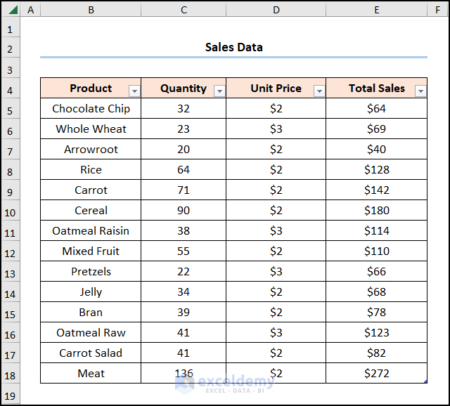
We have a sample Sales Dataset containing the “Product”, “Quantity”, “Unit Price” and “Total Sales” columns shown in cells B4:E18. We want to generate a dynamic list from a table in Excel using the Table feature and combining functions.
Method 1 – Creating Dynamic List Based on Cell Value
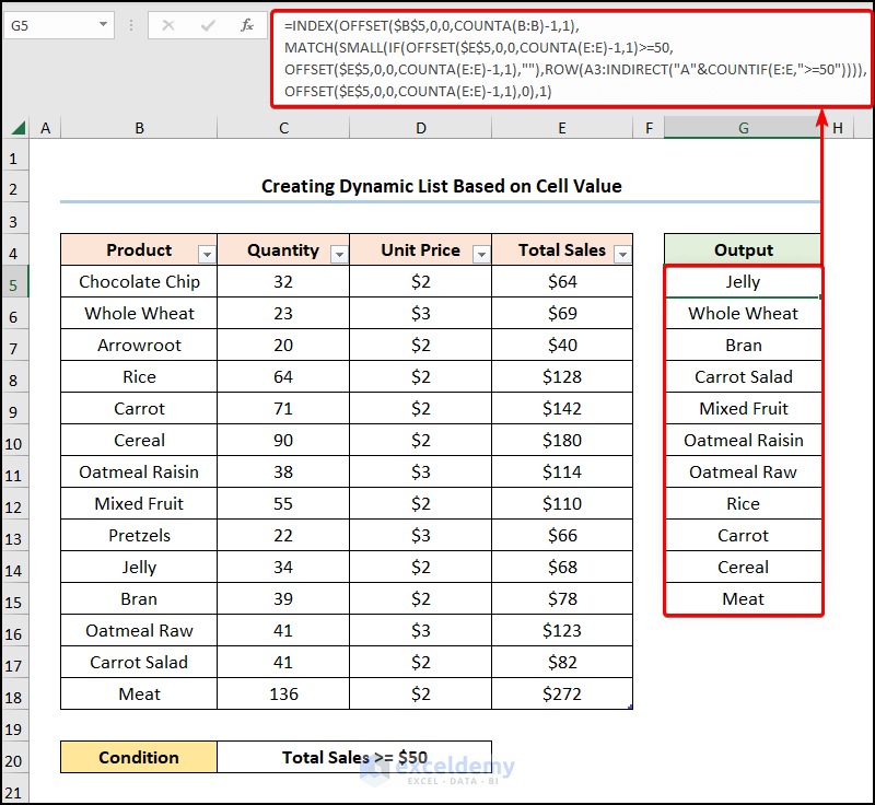
Let’s construct a dynamic list based on a given criterion. We will use the INDEX, MATCH, OFFSET, COUNTA, SMALL, IF, INDIRECT, COUNTIF, and ROW functions to obtain the “Product” names whose “Total Sales” value exceeds “$50”.
Steps:
- In cell G5 >> enter the formula given below >> click ENTER.
=INDEX(OFFSET($B$5,0,0,COUNTA(B:B)-1,1),MATCH(SMALL(IF(OFFSET($E$5,0,0,COUNTA(E:E)-1,1)>=50,OFFSET($E$5,0,0,COUNTA(E:E)-1,1),""),ROW(A3:INDIRECT("A"&COUNTIF(E:E,">=50")))),OFFSET($E$5,0,0,COUNTA(E:E)-1,1),0),1)
- OFFSET($E$5,0,0,COUNTA(E:E)-1,1) → returns a range of cells from the specified rows and columns. Where $E$5 is the reference argument, 0 is the rows argument which tells the function how many rows to move from the initial reference $E$5 and 0 represents the columns argument, which specifies the column from starting point. COUNTA(E:E)-1 is the optional height argument, which counts the number of non-blank cells in the range, while the 1 is the optional width argument.
- Output → {64;69;40;128;142;180;114;110;66;68;78;123;82;272}
- COUNTIF(E:E,”>=50″) → counts the number of cells within a range that meet the given condition. E:E cells represent the range argument that refers to the “Total Sales”, “>=50” indicates the criteria argument that returns the count of the matched value. We have taken the entire E column (E:E) instead of E5:E18 cells for making the list dynamic.
- Output → 13
- INDIRECT(“A”&COUNTIF(E:E,”>=50″)) → returns the reference specified by a text string. “A”&COUNTIF(E:E,”>=50″) is the ref_text argument.
- Output → 0
- ROW(A3:INDIRECT(“A”&COUNTIF(E:E,”>=50″))) → returns the serial number of the row.
- Output → {3;4;5;6;7;8;9;10;11;12;13}
- IF(OFFSET($E$5,0,0,COUNTA(E:E)-1,1)>=50,OFFSET($E$5,0,0,COUNTA(E:E)-1,1),””) → checks whether a condition is met and returns one value if TRUE and another value if FALSE. $E$5,0,0,COUNTA(E:E)-1,1)>=50 is the logical_test argument that selects the “Total Sales” values above “$50”. If this condition holds TRUE then the function returns OFFSET($E$5,0,0,COUNTA(E:E)-1,1) (value_if_true argument) otherwise it returns “” (Blank) (value_if_false argument).
- Output → {64;69;””;128;142;180;114;110;66;68;78;123;82;272}
- SMALL(IF(OFFSET($E$5,0,0,COUNTA(E:E)-1,1)>=50,OFFSET($E$5,0,0,COUNTA(E:E)-1,1),””),ROW(A3:INDIRECT(“A”&COUNTIF(E:E,”>=50″)))) → becomes
- SMALL({64;69;””;128;142;180;114;110;66;68;78;123;82;272},{3;4;5;6;7;8;9;10;11;12;13}) → returns the kth smallest value in data set. Here, {64;69;””;128;142;180;114;110;66;68;78;123;82;272} is the array argument while {3;4;5;6;7;8;9;10;11;12;13} is the k argument.
- Output → {68;69;78;82;110;114;123;128;142;180;272}
- MATCH(SMALL(IF(OFFSET($E$5,0,0,COUNTA(E:E)-1,1)>=50,OFFSET($E$5,0,0,COUNTA(E:E)-1,1),””),ROW(A3:INDIRECT(“A”&COUNTIF(E:E,”>=50″)))),OFFSET($E$5,0,0,COUNTA(E:E)-1,1),0) → becomes
- MATCH({68;69;78;82;110;114;123;128;142;180;272},{64;69;40;128;142;180;114;110;66;68;78;123;82;272},0) → returns the relative position of an item in an array matching the given value. Here, {68;69;78;82;110;114;123;128;142;180;272} is the lookup_value argument while {64;69;40;128;142;180;114;110;66;68;78;123;82;272} represents the lookup_array argument from where the value is matched. 0 is the optional match_type argument, which indicates the Exact match criteria.
- Output → {10;2;11;13;8;7;12;4;5;6;14}
- OFFSET($B$5,0,0,COUNTA(B:B)-1,1) → $B$5 is the reference argument, 0 is the rows argument which tells the function how many rows to move from the initial reference $E$5 and 0 represents the columns argument which specifies the column from starting point. COUNTA(B:B)-1 is the optional height argument, 1 is the optional width argument.
- Output → {“Chocolate Chip”;”Whole Wheat”;”Arrowroot”;”Rice”;”Carrot”;”Cereal”;”Oatmeal Raisin”;”Mixed Fruit”;”Pretzels”;”Jelly”;”Bran”;”Oatmeal Raw”;”Carrot Salad”;”Meat”;0;”Condition”}
- INDEX(OFFSET($B$5,0,0,COUNTA(B:B)-1,1),MATCH(SMALL(IF(OFFSET($E$5,0,0,COUNTA(E:E)-1,1)>=50,OFFSET($E$5,0,0,COUNTA(E:E)-1,1),””),ROW(A3:INDIRECT(“A”&COUNTIF(E:E,”>=50″)))),OFFSET($E$5,0,0,COUNTA(E:E)-1,1),0),1) → becomes
- INDEX({“Chocolate Chip”;”Whole Wheat”;”Arrowroot”;”Rice”;”Carrot”;”Cereal”;”Oatmeal Raisin”;”Mixed Fruit”;”Pretzels”;”Jelly”;”Bran”;”Oatmeal Raw”;”Carrot Salad”;”Meat”;0;”Condition”},{10;2;11;13;8;7;12;4;5;6;14},1) → returns a value at the intersection of a row and column in a given range. ({“Chocolate Chip”;”Whole Wheat”;”Arrowroot”;”Rice”;”Carrot”;”Cereal”;”Oatmeal Raisin”;”Mixed Fruit”;”Pretzels”;”Jelly”;”Bran”;”Oatmeal Raw”;”Carrot Salad”;”Meat”;0;”Condition”} is the array argument that are the “Product” names. {10;2;11;13;8;7;12;4;5;6;14} is the row_num argument that indicates the row location. 1 is the optional column_num argument that points to the column location.
Read More: How to Create Dynamic List in Excel Based on Criteria
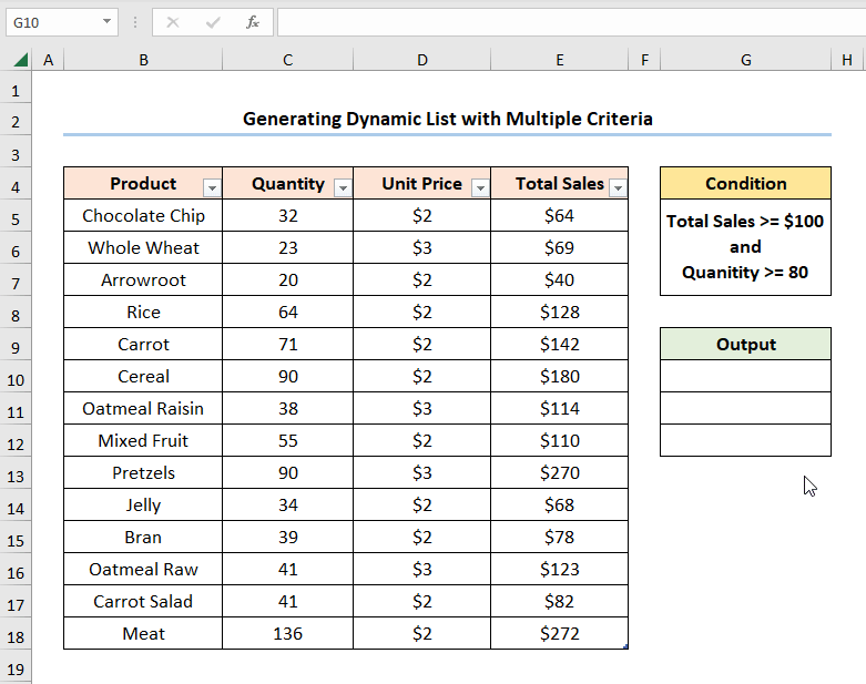
Method 2 – Generating Dynamic List with Multiple Criteria
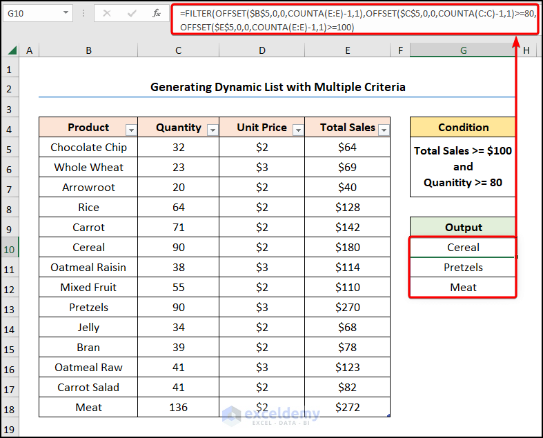
We want to extract the “Product” names which sold over “80” units in “Quantity” and generated “Total Sales” greater than “$100”.
Steps:
- Select cell G10>> enter the following expression >> press ENTER.
=FILTER(OFFSET($B$5,0,0,COUNTA(E:E)-1,1),OFFSET($C$5,0,0,COUNTA(C:C)-1,1)>=80,OFFSET($E$5,0,0,COUNTA(E:E)-1,1)>=100)
- OFFSET($C$5,0,0,COUNTA(C:C)-1,1)>=80 → the function returns TRUE or FALSE for the “Quantity” values greater than “80”.
- Output → {FALSE;FALSE;FALSE;FALSE;FALSE;TRUE;FALSE;FALSE;TRUE;FALSE;FALSE;FALSE;FALSE;TRUE}
- OFFSET($E$5,0,0,COUNTA(E:E)-1,1)>=100 → the function returns TRUE or FALSE for the “Total Sales” greater than “$100”.
- Output → {FALSE;FALSE;FALSE;TRUE;TRUE;TRUE;TRUE;TRUE;TRUE;FALSE;FALSE;TRUE;FALSE;TRUE}
- FILTER(OFFSET($B$5,0,0,COUNTA(E:E)-1,1),OFFSET($C$5,0,0,COUNTA(C:C)-1,1)>=80,OFFSET($E$5,0,0,COUNTA(E:E)-1,1)>=100) → filter a range or array. OFFSET($B$5,0,0,COUNTA(E:E)-1,1) is the array argument, OFFSET($C$5,0,0,COUNTA(C:C)-1,1)>=80 is the include argument. OFFSET($E$5,0,0,COUNTA(E:E)-1,1)>=100 is the optional if_empty argument. The function returns the “Product Names” that match both these criteria.
- Output → {“Cereal”;”Pretzels”;”Meat”}
Read More: How to Create a Dynamic Top 10 List in Excel
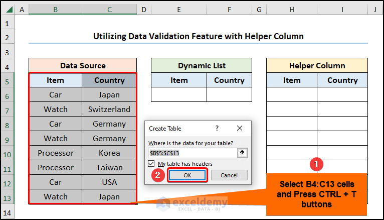
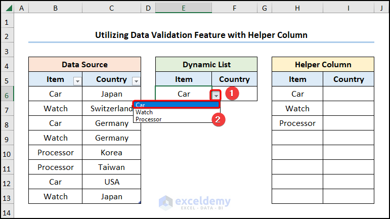
Method 3 – Utilizing Data Validation Feature with Helper Column
Steps:
- Select the range B5:C13>> click the CTRL + T keys to create Excel Table >> press OK.
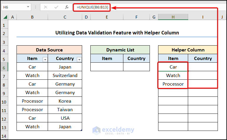
- Go to cell H6>> use the UNIQUE function to return the unique values in the B6:B13 range.
=UNIQUE(B6:B13)
The B6:B13 cells represent the “Item” column.
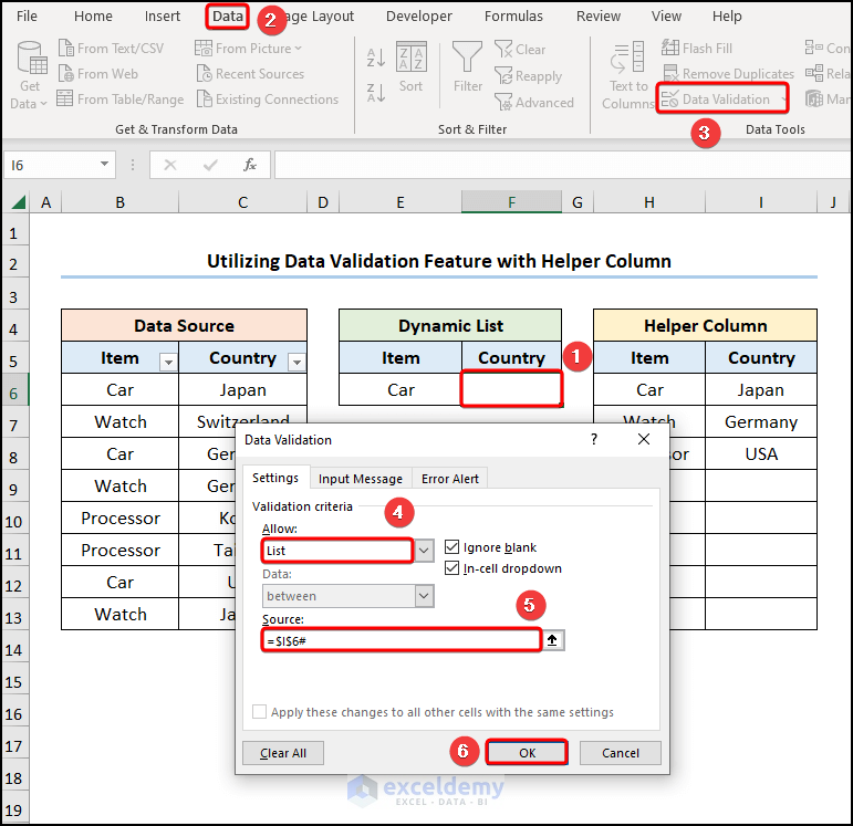
- Select the cell E6>> navigate to the Data tab >> click the Data Validation option.
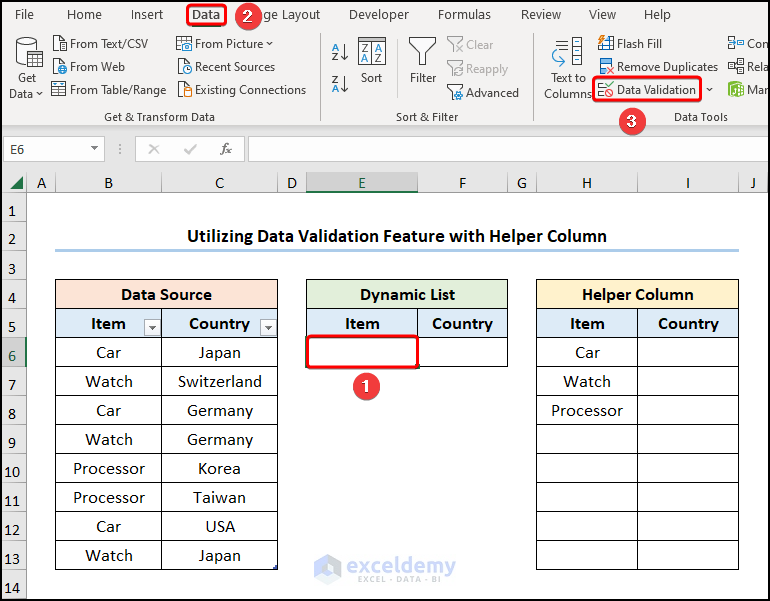
This opens the Data Validation window.
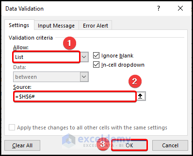
- In the Allow field, choose the List option >> enter the formula below in the Source field >> hit OK.
$H$6#
The H6 cell points to “Item” in the “Helper Column” while the # (Hashtag) sign indicates the Spill Range.
- Click the Down arrow >> select an “Item” from the list, here we’ve chosen “Car”.
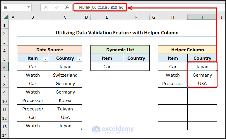
- Go to cell I6>> insert the FILTER function to filter the array. The “Country” corresponding to each “Item” is shown.
=FILTER(C6:C13,B6:B13=E6)
The C6:C13 and B6:B13 ranges point to the “Item” and “Country” columns, while the E6 cell refers to the “Item” chosen from the Data Validation drop-down.
- Insert another drop-down in the F6 cell by entering the following formula.
$I$6#
Cell I6 represents the “Country” in the “Helper Column” and the # (Hashtag) sign refers to the Spill Range.
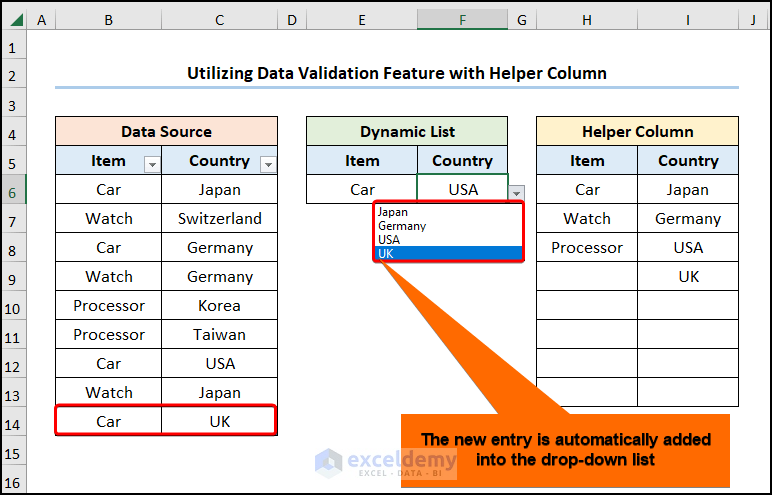
Adding new data updates the dynamic drop-down list, as shown in the image below.
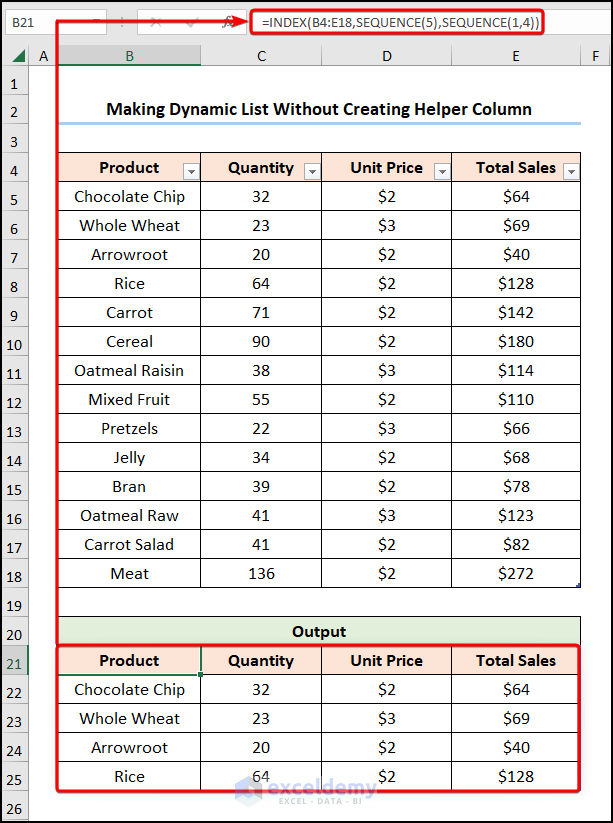
Method 4 – Making Dynamic List Without Creating Helper Column
Steps:
- Enter the following formula in cell B21>> click ENTER.
=INDEX(B4:E18,SEQUENCE(5),SEQUENCE(1,4))
- INDEX(B4:E18,SEQUENCE(5),SEQUENCE(1,4))
- SEQUENCE(5) → returns a sequence of numbers. 5 is the rows argument.
- Output → {1;2;3;4;5}
- SEQUENCE(1,4) → here, 1 is the rows argument while 4 is the optional columns argument.
- Output → {1;2;3;4}
- INDEX(B4:E18,SEQUENCE(5),SEQUENCE(1,4)) → becomes
- INDEX(B4:E18,{1;2;3;4;5},{1;2;3;4}) → returns a value at the intersection of a row and column in a given range. B4:E18 is the array argument representing the dataset while {1;2;3;4;5} is the row_num argument that returns the first 5 rows and {1;2;3;4} is the optional column_num argument that indicates the location of the columns.
Read More: How to Make Dynamic Drop Down List from Another Sheet in Excel
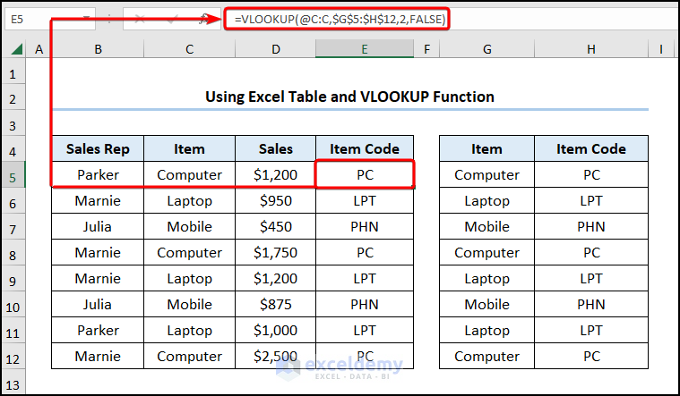
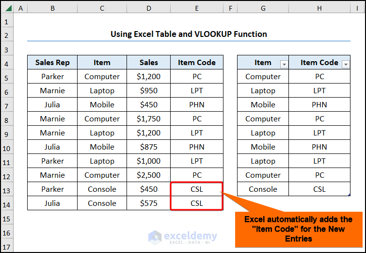
Method 5 – Using Excel Table and VLOOKUP Function
Steps:
- Go to cell E5 >> enter the equation into the Formula Bar >> press ENTER >> drag the Fill Handle tool to copy the formula into the cells below.
<span style="font-size: 14pt;">=VLOOKUP(@C:C,$G$5:$H$13,2,FALSE)</span>
- VLOOKUP(@C:C,$G$5:$H$13,2,FALSE) → @C:C ( lookup_value argument) is mapped from the $G$5:$H$13 (table_array argument) array. 2 (col_index_num argument) represents the column number of the lookup value. FALSE (range_lookup argument) refers to the Exact match of the lookup value.
- Output → PC
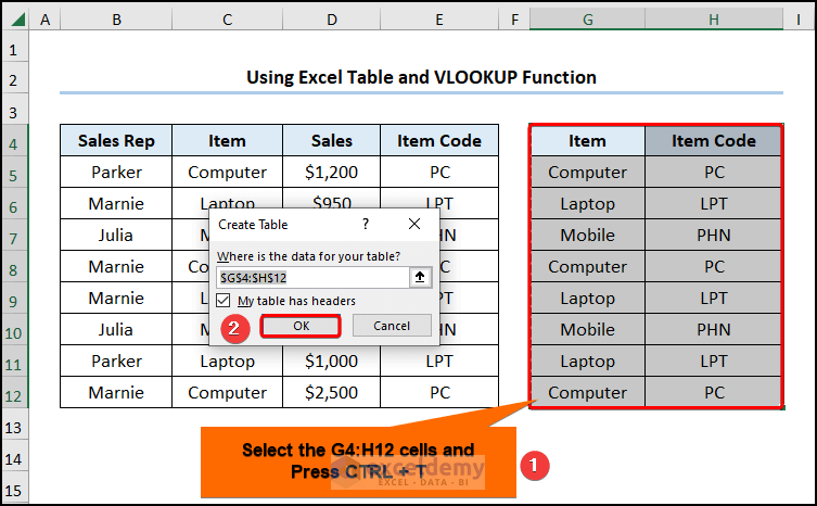
- Select the G4:H12 array >> press the CTRL + T shortcut keys to insert Excel Table >> press OK.
- Add a new “Item” and its “Item Code” as shown below.
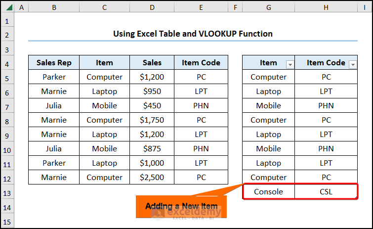
- When we enter new data into the dataset, Excel dynamically inserts the “Item Code”.
Read More: How to Create Dynamic Drop Down List Using Excel OFFSET
Download Practice Workbook
<< Go Back to Dynamic List Excel | Excel Drop-Down List | Data Validation in Excel | Learn Excel
Get FREE Advanced Excel Exercises with Solutions!
