Method 1 – Creating a Drop-Down List in Excel
The dataset contains some candidate names in column B. We’ll create a drop-down that inputs one of three values in the cells of column C.
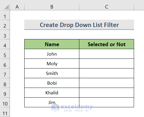
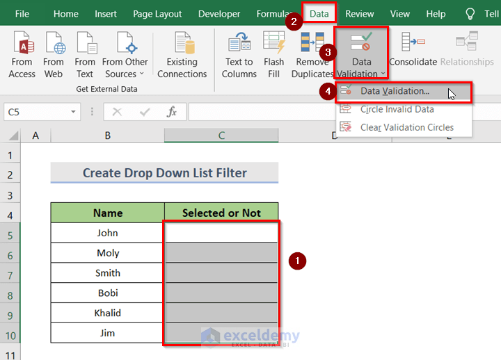
- Select the cells where you want to create the drop-down list filter.
- Click on the Data tab on the ribbon.
- Go to the Data Validation drop-down menu.
- Select Data Validation from the drop-down menu.
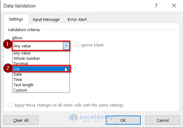
- This will open the Data Validation dialog box.
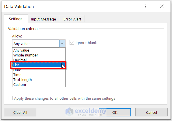
- In the Settings option, click on the drop-down menu under Allow.
- By default, Any value is selected. Change it to List.
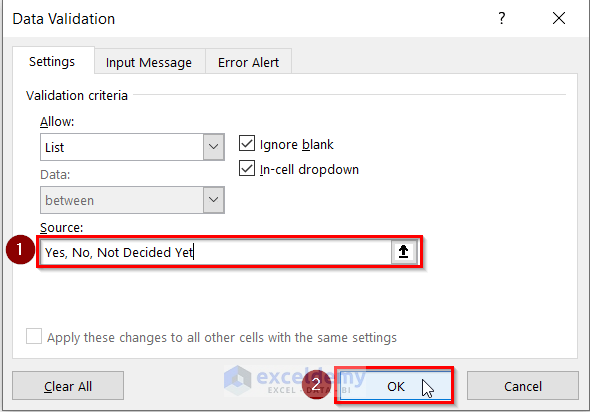
- This will show a box named Source. Write Yes, No, Not Decided Yet in the source box.
- Click on the OK button.
- The selected cells are now drop-down list boxes.
- Make a list of who is selected.
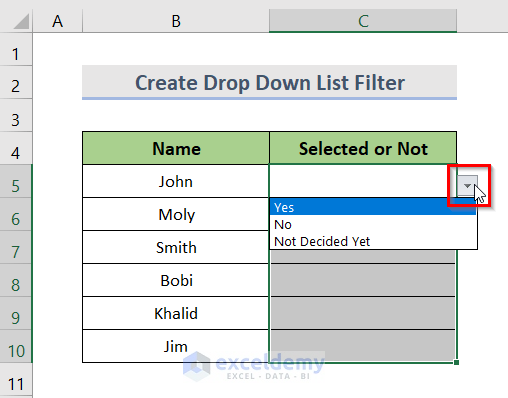
- You can change the data by clicking on the list and selecting a value.

Read More: How to Make a Drop Down List in Excel
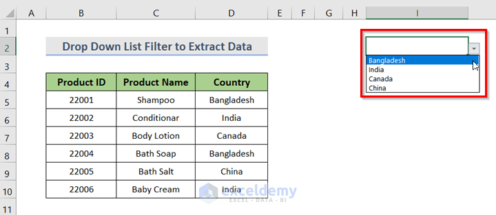
Method 2 – Creating an Excel Drop Down List Filter to Extract Data
We have a dataset that contains product IDs in column B, the name of the products in column C, and the country name in column D.

Part 2.1 – Making a List of Unique Items
STEPS:
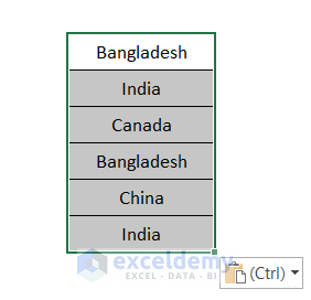
- Select the countries in column D.
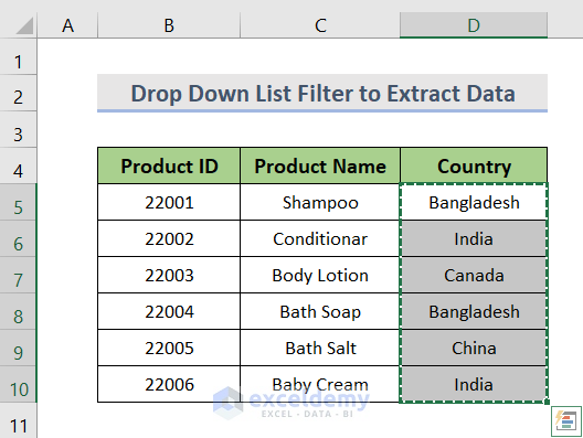
- Paste the selection anywhere else in the worksheet.
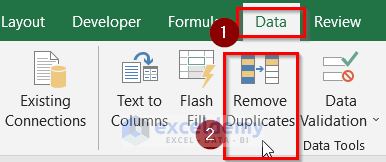
- Go to the Data tab from the ribbon.
- Click on Remove Duplicates.
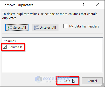
- You will get the Remove Duplicates dialog box.
- Check the column.
- Click OK.
- A pop-up window will appear, confirming that the duplicate values were removed from the selected column.
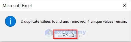
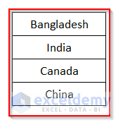
- We can see that 2 duplicate values are removed and 4 unique values are remaining.
Part 2.2 – Putting a Drop-Down Filter to Show Unique Items
STEPS:
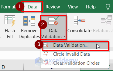
- Go to the Data tab.
- Click on the Data Validation drop-down menu.
- Select Data Validation.
- The Data Validation dialog box will appear.
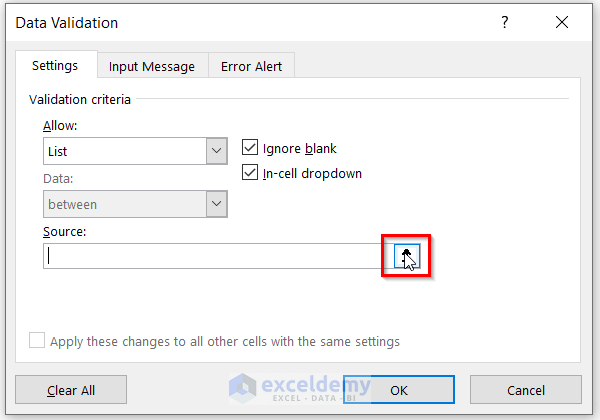
- Select List from the drop-down.
- Click on the arrow in the Source section.
- Select the unique values that were generated in the previous part.
- Hit Enter.
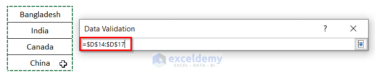
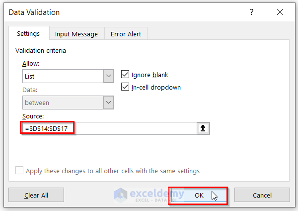
- The reference to the unique values is in the source section.
- Click OK.
- The drop-down list is now shown in I2.
Read More: How to Create a Drop Down List with Unique Values in Excel
Part 2.3 – Using Helper Columns to Extract Records
STEPS:
- In the first helper column, we need the row number for each of these cells. So, E5 would be row number 1 in the dataset and E6 would be row number 2. Input these values manually or use the ROWS function:
=ROWS($D$5:D5)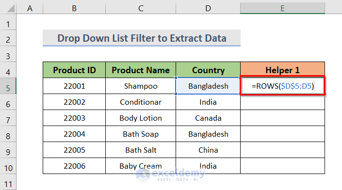
- Press Enter.
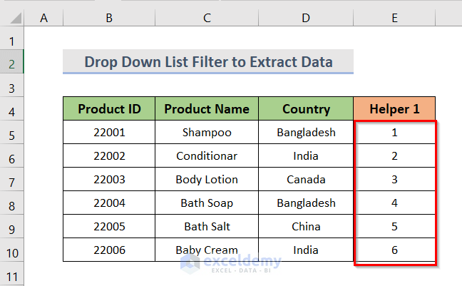
- Drag the fill handle to copy the formula to show all the rows.
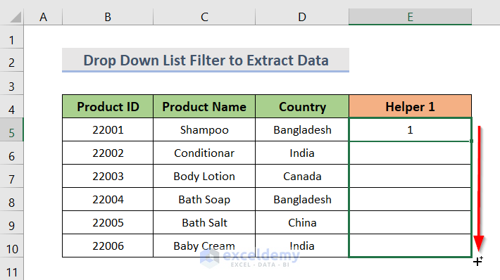
- The cells are incremented automatically.
- Create a helper column which only shows those row numbers which match the country that was selected in I2.
- Insert the following formula in F5:
=IF($I$2=D5,E5,"")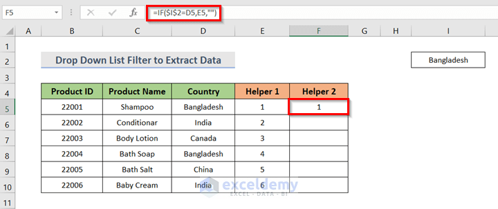
- Drag the fill handle down to show the numbers.
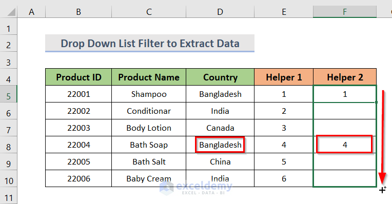
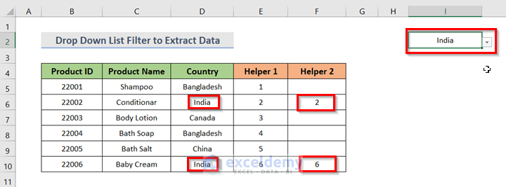
- If we change the country, we can see the helper column will show the row number that contains the country.
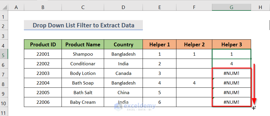
- We need another helper column G
- Insert the formula below in G5:
=SMALL($F$5:$F$10,ROWS($F$5:F5))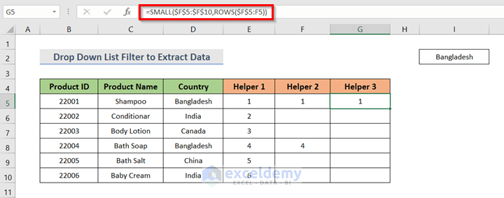
We use ROWS($F$5:F5) to return the first smallest value.
- When we drag the Fill Handle down, it shows #NUM! errors.
- Replace the original formula with the following:
=IFERROR(SMALL($F$5:$F$10,ROWS($F$5:F5)),"")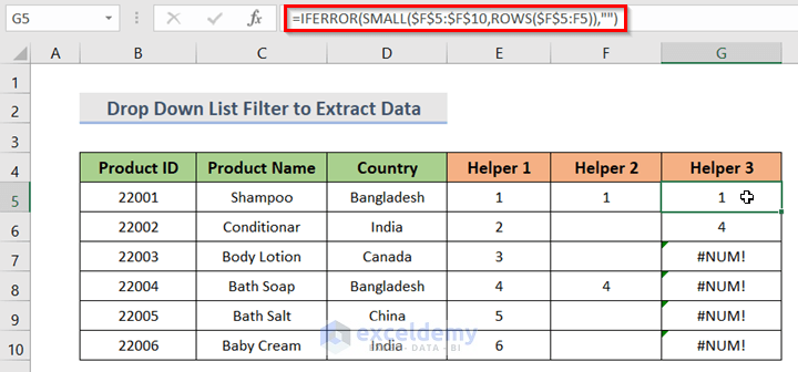
The IFERROR function will remove the error.
- When we drag the fill handle, the row numbers will show properly.
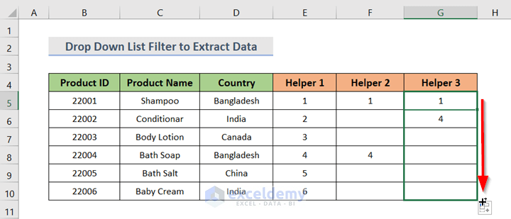
- The three columns show the selected countries’ product IDs and product names.
- In cell K5, use this formula:
=INDEX($B$5:$D$10,$G5,COLUMNS($H$5:H5))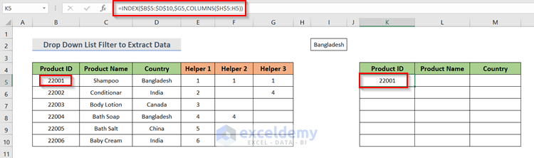
In the COLUMNS($H$5:H5), select the same column which is in the left parenthesis of the worksheet.
- The #VALUE! error is showing up.
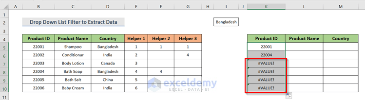
- Replace the formula in the K column with:
=IFERROR(INDEX($B$5:$D$10,$G5,COLUMNS($H$5:H5)),"")![]()
- Drag the fill handle over K5:M10.
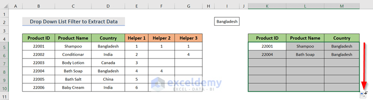
- Hide the helper columns if you want.
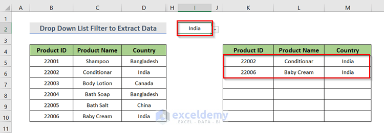
- If we change the country from the drop-down filter list, the table on the right changes automatically.
Method 3 – Sorting and Filtering Data from an Excel Drop-Down List
We are going to use the same dataset, with product ID, product name, and country.
Part 3.1 – Creating a Drop-Down List Using the Sort and Filter Feature
STEPS:
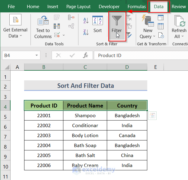
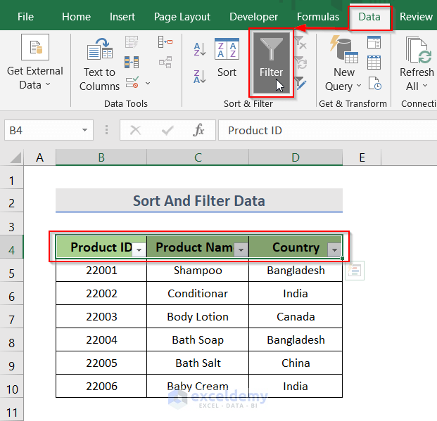
- Select the headers of the dataset.
- From the Data tab on the ribbon, click on Filter in the Sort & Filter section.
- This makes all the headers get a drop-down filter arrow.
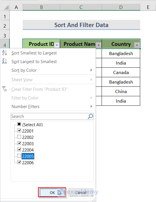
- Click on any of the headers that we want to filter out. We clicked on the Product ID drop-down arrow to filter out the products.
- Uncheck the data you don’t want to view.
- Click on the OK button.
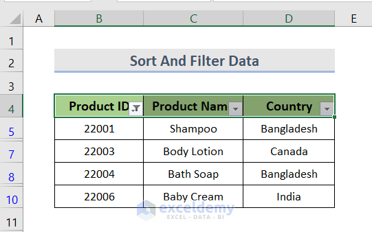
- All the unchecked products are now hidden.
Part 3.2 – Adding a New Filter
STEPS:
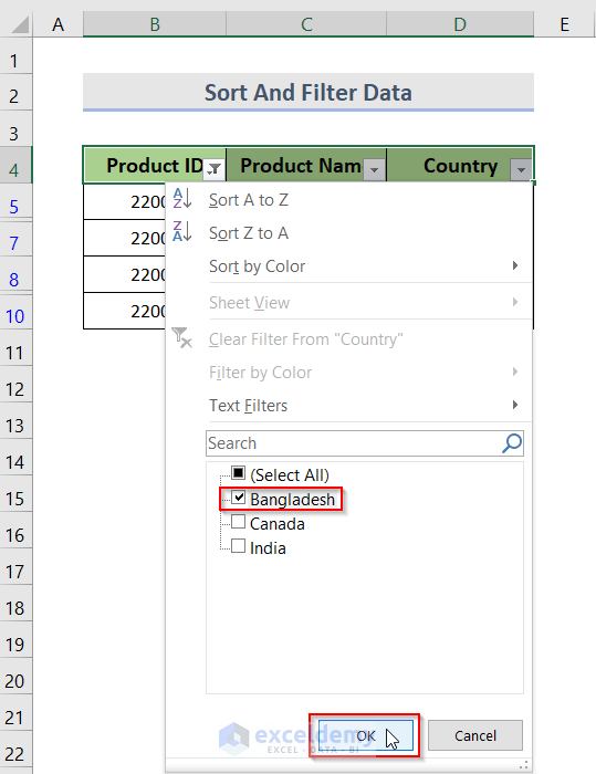
- Click the drop-down arrow to add new filters. We will click on the country column.
- Uncheck all the countries you don’t want to view. We chose to leave Bangladesh.
- Click OK.
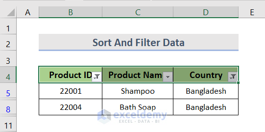
- Only the products from the country Bangladesh are now visible. Others are temporarily hidden.
Part 3.3 – Clearing an Existing Filter
STEPS:
- Click on the header drop-down arrow which is filtered. We want to clear the filter from product identification.
- Click on Clear Filter From “Product ID”.
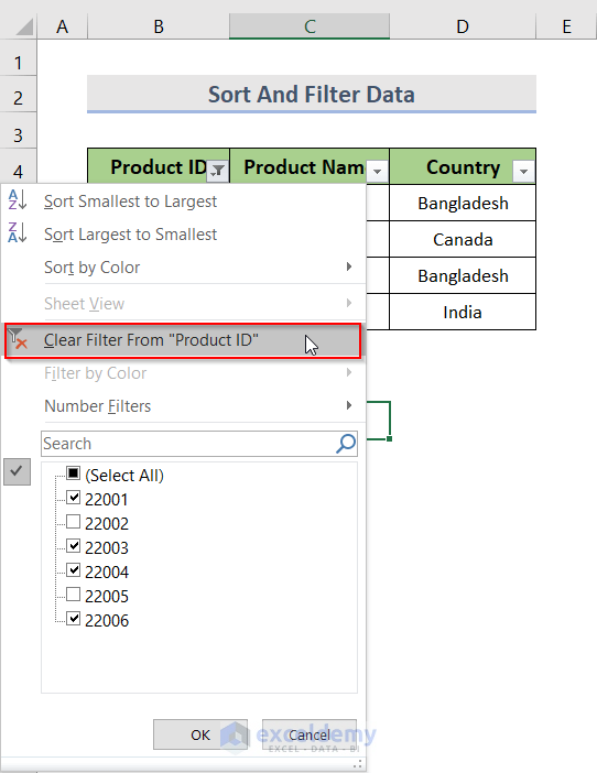
- The drop-down list filters are removed now.
Read More: How to Add Item to Drop-Down List in Excel
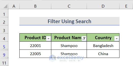
Method 4 – Filtering Data in Excel Using Search
STEPS:
- Select all the headers you want to make a drop-down box for.
- Go to the Data tab and click on Filter.
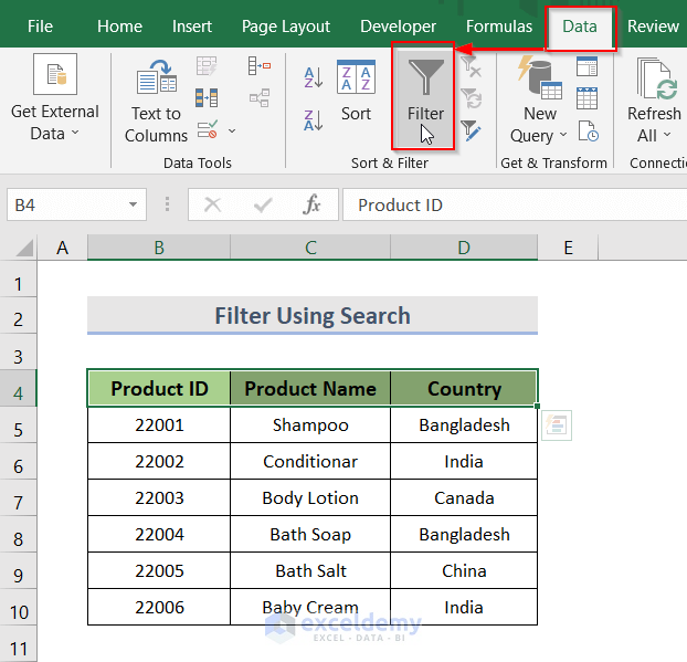
- To filter a column, click the drop-down arrow in that column. We want to filter the product name column.
- In the search box shown in the picture, write down the product name. We wrote Shampoo.
- Click OK.
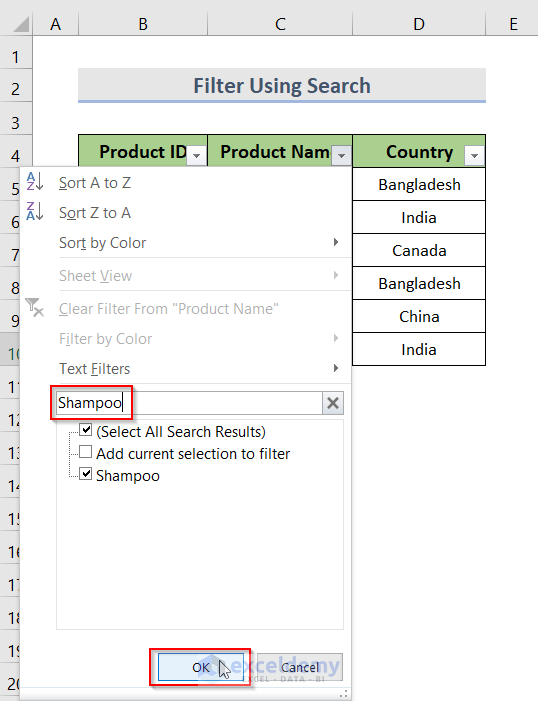
- Excel will display only the data that contains the product name Shampoo.
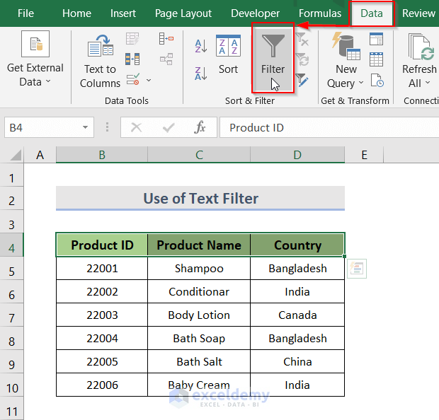
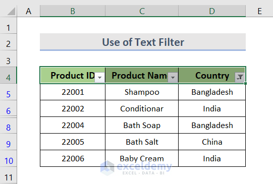
Method 5 – Applying Text Filters in an Excel Drop-Down List Filter
STEPS:
- To construct a drop-down box, choose all of the headings of the dataset.
- Go to the Data tab and select Filter.
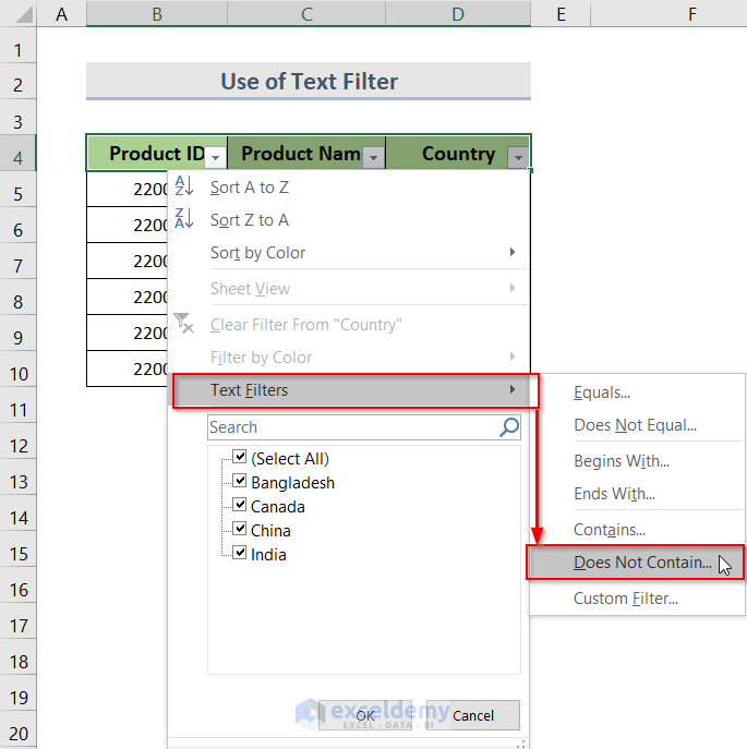
- Click on the drop-down arrow in the column of the text you want to filter. We clicked on the country column.
- Go to Text Filters and select Do Not Contain.
- A Custom AutoFilter dialog box will appear. We don’t want any data with Canada, so we selected Canada.
- Click OK.
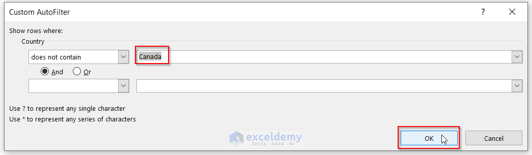
- This filters out rows with Canada.
Read More: How to Auto Update Drop-Down List in Excel
Method 6 – Using Number Filtering in an Excel Drop-Down List Filter
STEPS:
- Select the headers.
- Go to the Data tab and click on Filter.
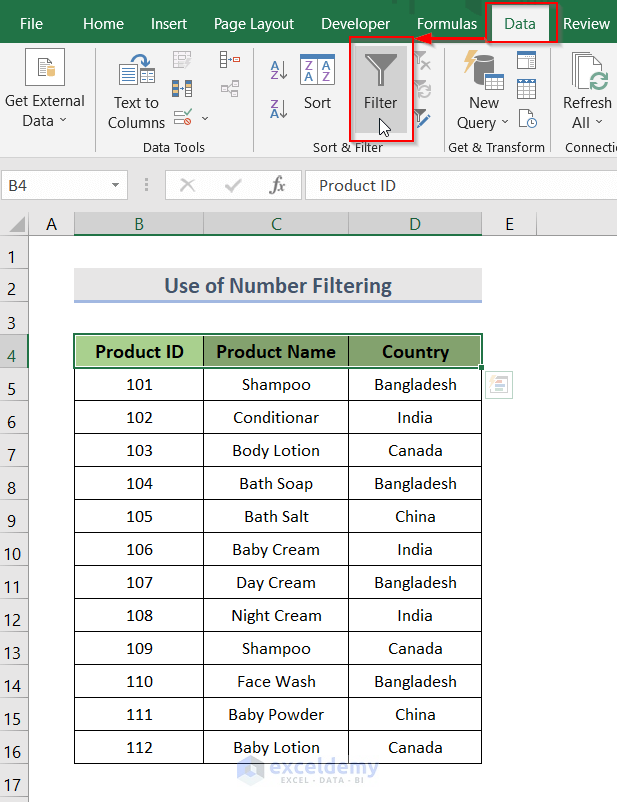
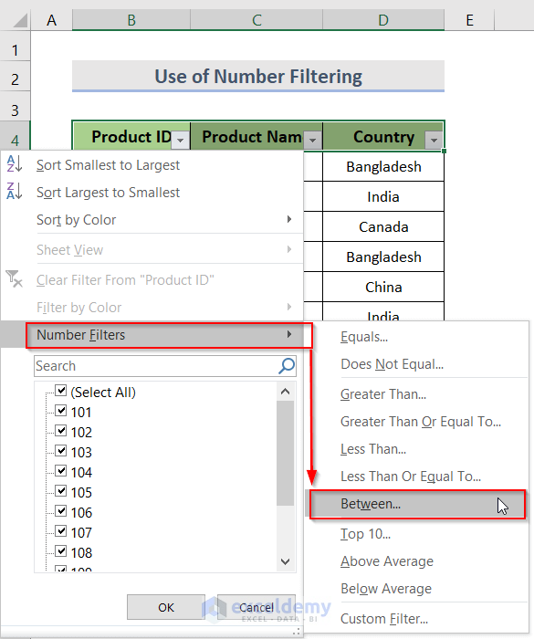
- Click on the drop-down arrow of the column which contains the numbers. We will click on product identification.
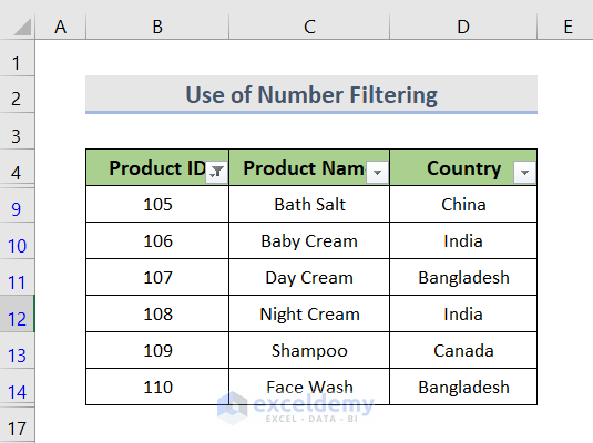
- From Number Filters, select Between. We want to see the products with IDs between 105 and 110.
- This will open up the Custom AutoFilter dialog box.
- Insert the numbers you want to filter by and choose the appropriate settings on the left.
- Click OK.
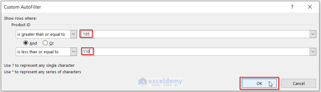
- The data is filtered to show Product IDs between 105 and 110.
Method 7 – Using Date Filters in an Excel Drop-Down List
STEPS:
- Select the headers.
- From the Data tab, click on Filter.
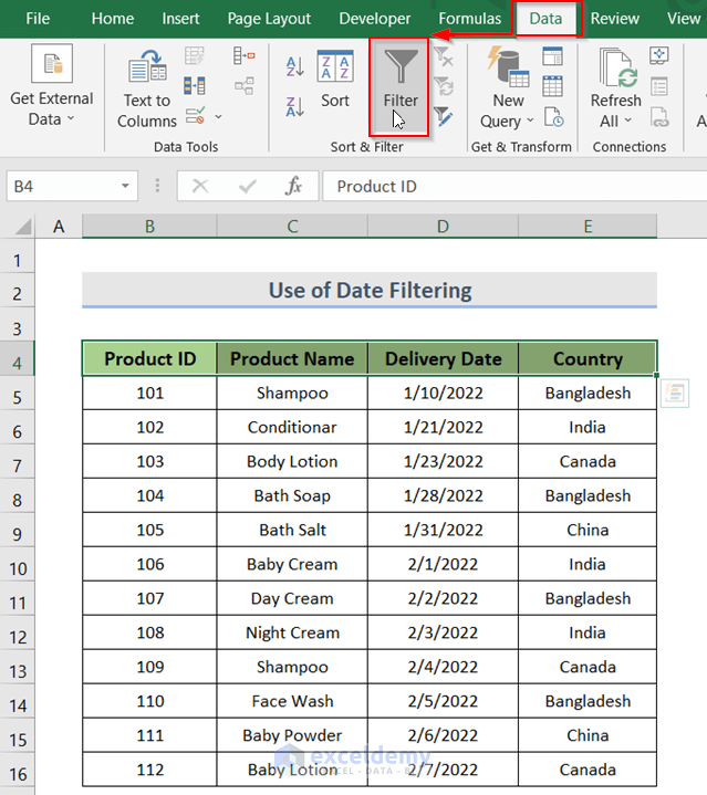
- Click on the Delivery date drop-down arrow.
- Go to Date Filters. We have selected last month.
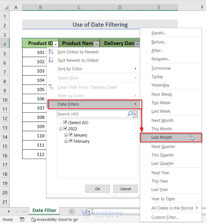
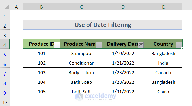
- All the products which were delivered in the last month are displayed.
Download the Practice Workbook
Excel Drop Down List Filter: Knowledge Hub
- Excel Data Validation Drop Down List with Filter
- How to Copy Filter Drop-Down List in Excel
- Excel Filter Drop-Down List Based on Cell Value
<< Go Back to Excel Drop-Down List | Data Validation in Excel | Learn Excel
Get FREE Advanced Excel Exercises with Solutions!
