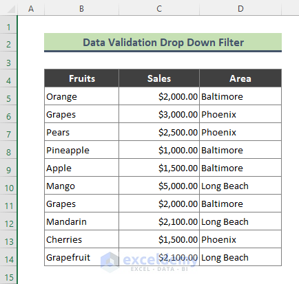
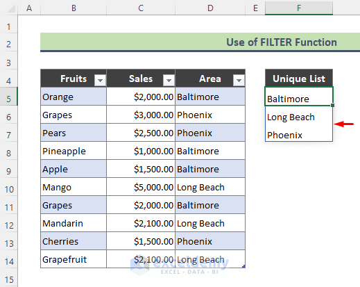
Let’s consider a dataset containing area-wise sales data of several fruits. We will create a Data Validation drop-down list of areas mentioned in the dataset and use the list to draw fruit sales data.
Method 1 – Filter Values from the Data Validation Drop Down List Using Helper Columns
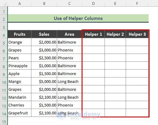
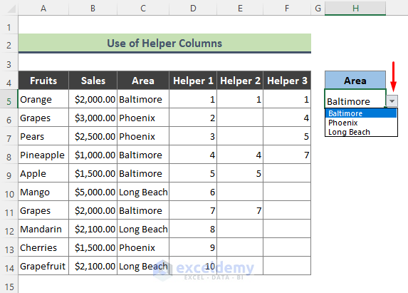
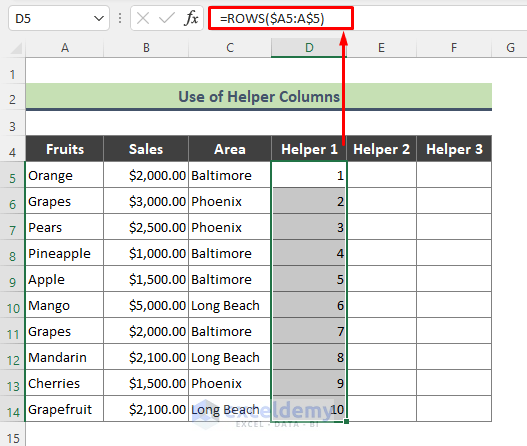
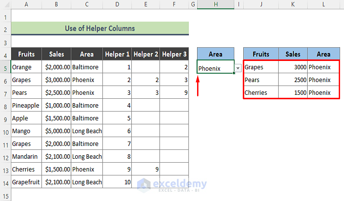
Let’s add three helper columns to the dataset which will be used to pull data.
Steps:
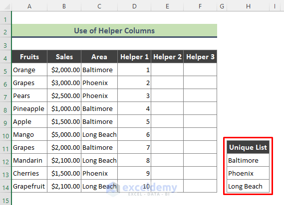
- List all the unique Areas separately.
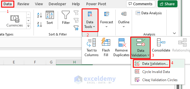
- Click on the cell where you want to put the drop-down list (here Cell H5).
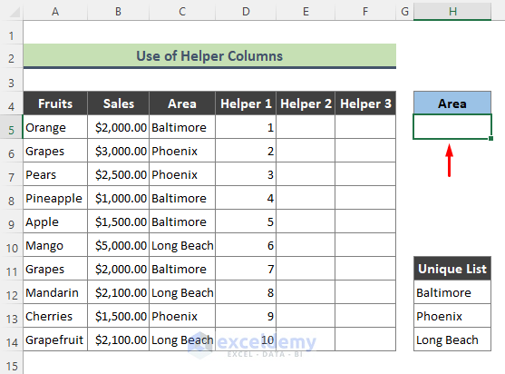
- From the Excel Ribbon, go to Data and Data Tools, then select Data Validation and choose the Data Validation option.
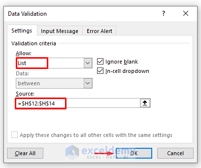
- The Data Validation dialog box will appear. Go to the Settings tab, choose List from Allow section and specify the Source as the unique list you created.
- Press OK.
- You’ll receive a drop-down list.
- Copy the following formula in the first helper column (in Cell D5). Press Enter and use the Fill Handle (+) tool to copy the formula over the entire column.
=ROWS($A5:A$5)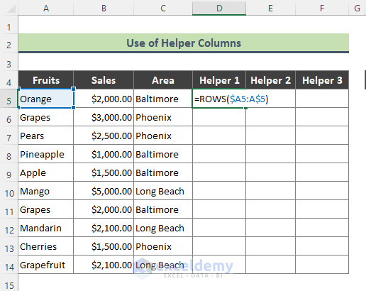
- You will get a simple array.
- Copy the following IF function for the second helper column (Helper 2):
=IF(C5=$H$5,D5,"")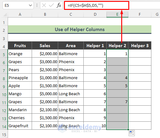
- For the third helper column (Helper 3), use the following formula:
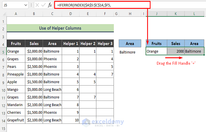
=IFERROR(SMALL($E$5:$E$14,D5),"")
Here, the SMALL function returns k-th smallest values in the range E5:E14. Later, the IFERROR function returns blank if the result of the SMALL formula is an error.
- Copy the following formula in Cell J5 and press Enter.
=IFERROR(INDEX($A$5:$C$14,$F5,COLUMNS($J$5:J5)),"")
Here, the INDEX function draws the data based on the wow number. Then the COLUMNS function returns the column number in the range $J$5:J5. Finally, the IFERROR function returns blank if the result is an error.
- Drag the Fill Handle two cells to the right to get all the data in a row.
- Drag the Fill Handle down for as many rows as you have in the original table (to ensure you get all the results).
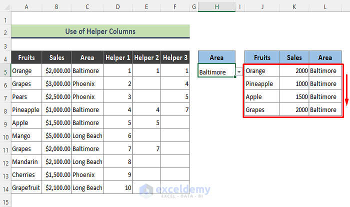
- If you choose the Phoenix area from the drop-down list, rows corresponding to Phoenix will be filtered as below.
Read More: How to Make a Data Validation List from Table in Excel
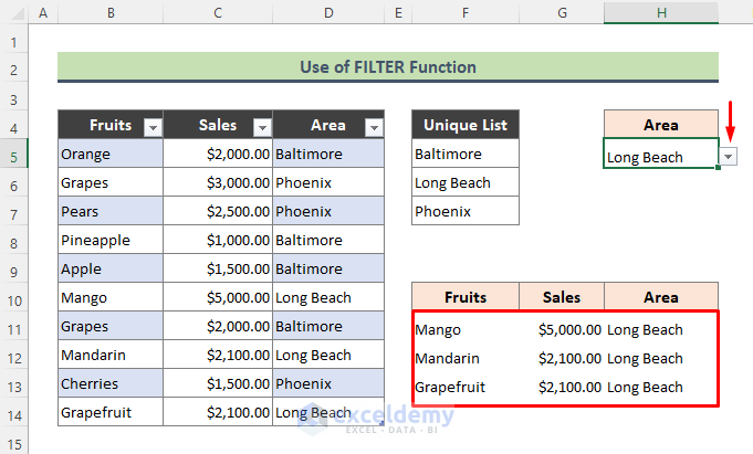
Method 2 – Use the Excel FILTER Function to Extract Data Based on a Data Validation Drop Down List
If you are working in Excel 2019 and later versions or in Microsoft 365, you can filter data using the FILTER function.
Steps:
- We converted the data range to an Excel table by pressing Ctrl + T. If you add new records to a table, the drop-down list gets updated according to the newly added data.
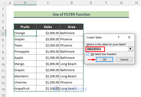
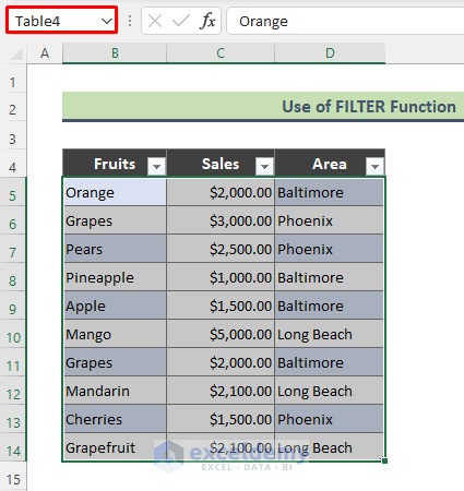
- Provide a name to the newly created table (say, Table4).
- Copy the following formula in Cell F5 and hit Enter.
=SORT(UNIQUE(Table4[Area]))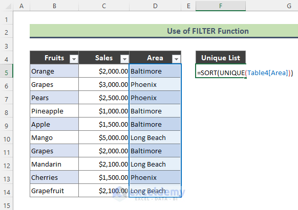
Here, I have used the SORT function along with the UNIQUE function to sort the above Area data.
- The above formula returns sorted unique data as an array (outlined in blue).
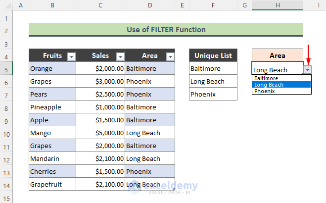
- Create the drop-down list in Cell H5 (choose Data Validation in the Data tab).
- From the Data Validation dialog box, choose List from Allow section and input the following formula in the Source field:
=F5#- Press OK.
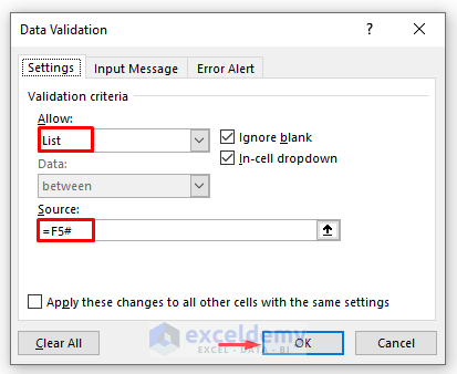
The # symbol indicates we are considering the whole array of Cell F5 as the source for the drop-down list.
- This creates a drop-down validator.
- Copy the following formula in Cell F11 and press Enter.
=FILTER(Table4,Table4[Area]=H5,"No Data Found")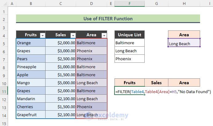
- Drag the fill handle to the right to show the results in all columns, then drag it down to cover more rows.
- Change the area from the drop-down list and thus filter the corresponding rows based on the area selected.
Read More: How to Use Data Validation List from Another Sheet
Download Practice Workbook
You can download the practice workbook that we have used to prepare this article.
Related Articles
<< Go Back to Excel Drop Down List Filter | Excel Drop-Down List | Data Validation in Excel | Learn Excel
Get FREE Advanced Excel Exercises with Solutions!
