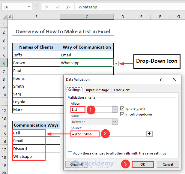
In the following overview image, we selected a range as the source in the Data Validation dialog to create a drop-down list.
⏷Ways of Making Drop-Down List in Excel
⏵Insert List Values Manually
⏵Insert List Values from a Range of Cells
⏵Apply Name Manager
⏵Combine Table Tool and INDIRECT Function
⏵Apply OFFSET Function
⏷Copy and Paste a Drop-Down List to Other Cells
⏵Use Keyboard Shortcut
⏵Apply Paste Special Command
⏷Make a Dependent Drop-Down List
⏷Make an Editable Drop-Down List
⏷Make a Dynamic Drop-Down List
⏵Use OFFSET and COUNTA Functions
⏵Use OFFSET and COUNTIF Functions
⏷Add or Remove Items from a Drop-Down List Without Opening Data Validation
⏵Add Items Using Insert Command from Context Menu
⏵Remove Items Using Delete Command from Context Menu
⏷Input a Message in a Drop-Down List
⏷Put an Error Alert in Excel Drop-Down List
⏷Protect Your Drop-Down List
⏷Make a Custom List in Excel
⏵Use Pre-Existing List
⏵Manually Create a List
⏷Make a Unique List
⏷Import a List in Excel
⏵Import a Custom List from Another Worksheet
⏵Import a Drop-Down List from Another Workbook
⏷Make a Numbered List in Excel
⏵Use Auto Fill Feature (Static Numbered List)
⏵Use Fill Handle Tool
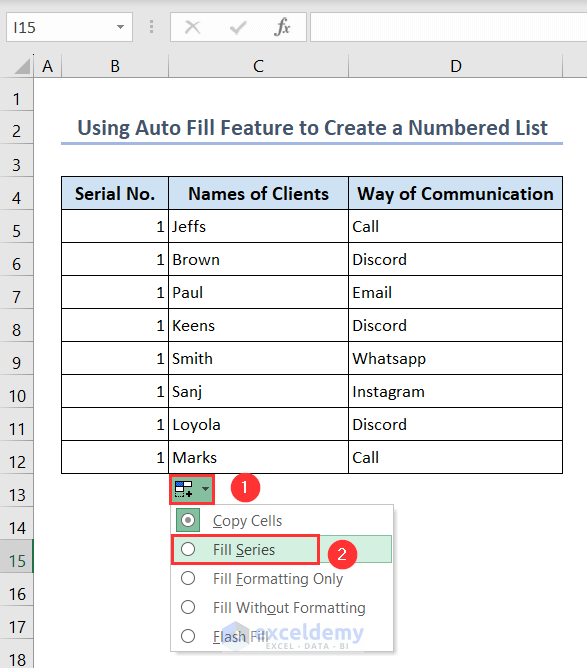
⏵Use Fill series Option
⏵Use ROW Function
⏵Use ROW Function in an Excel Table (Dynamic Numbered List)
⏵Use ROWS and SEQUENCE Functions (Dynamic Numbered List)
⏷Make a Bulleted Number List
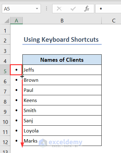
⏵Use Keyboard Shortcuts
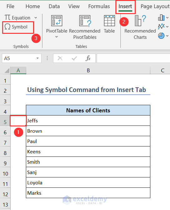
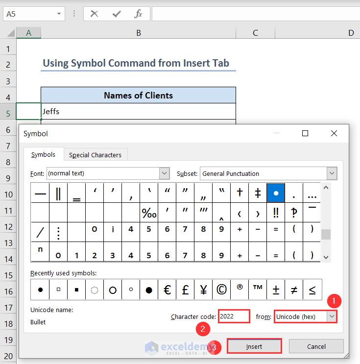
⏵Use Symbol Command
⏵Use Custom Format
⏵Copying and Pasting from Word
⏵Use CHAR Function and Ampersand Operator
⏵Use Wingdings Font
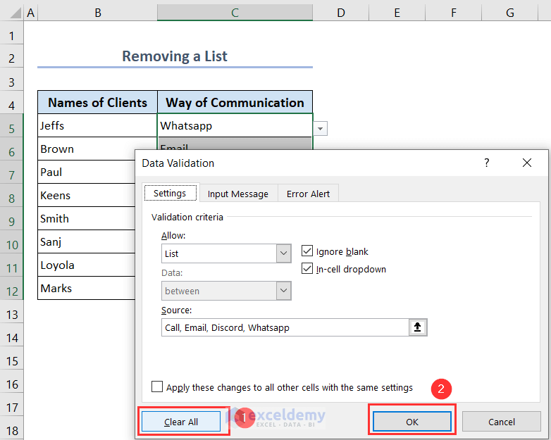
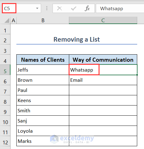
⏷Remove a List from Excel
⏷Things to Remember
⏷Frequently Asked Questions
⏷Make List in Excel: Knowledge Hub
How to Make a Drop-Down List in Excel
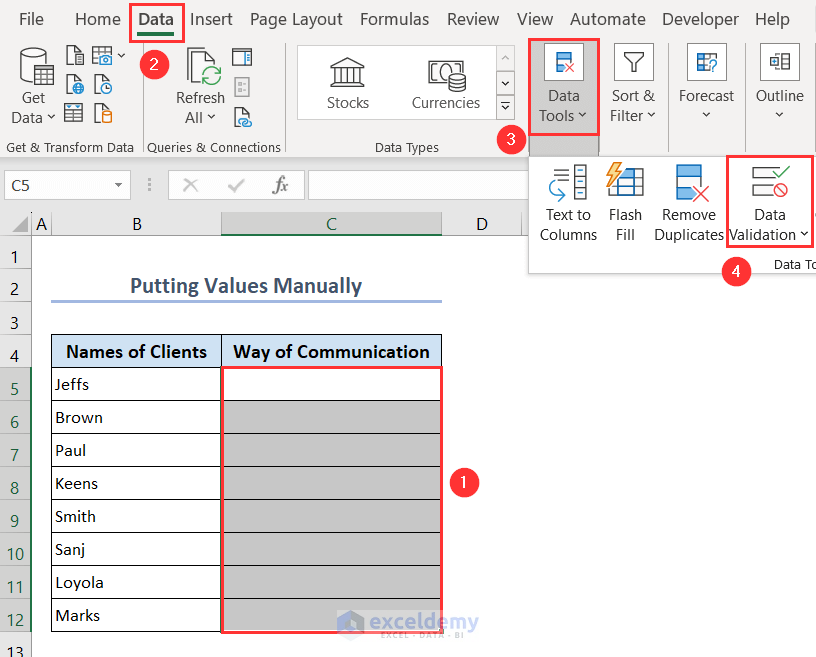
Method 1 – Insert List Values Manually in Data Validation to Make a Drop-Down List
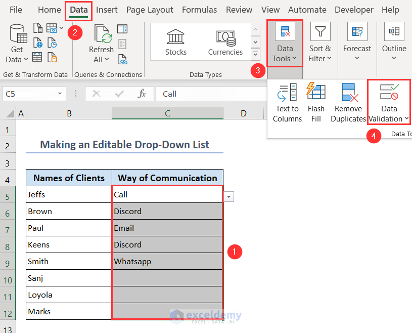
- Select all the cells from C5:C12 and go to Data, then go to Data Tools and select Data Validation.
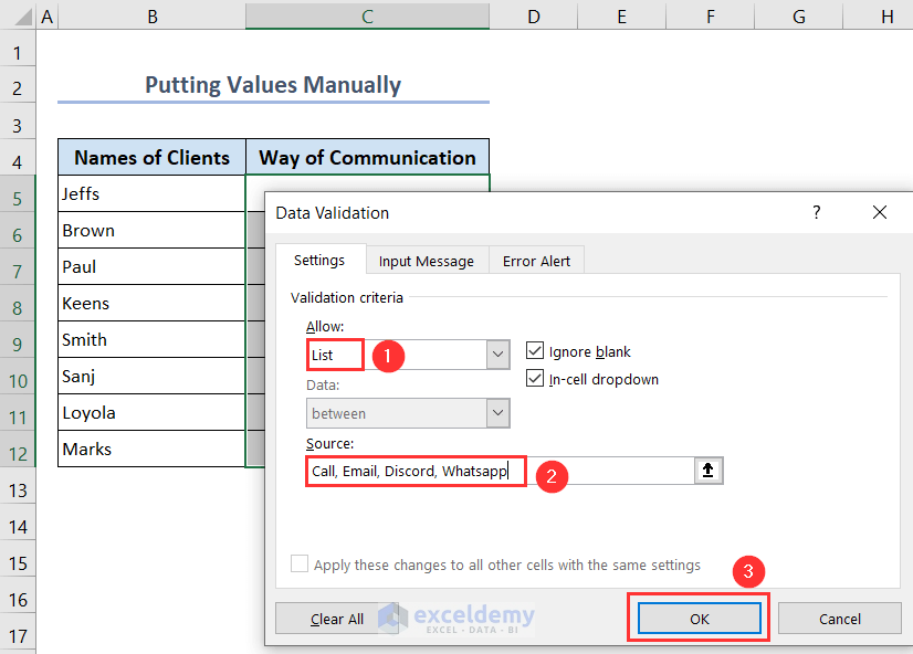
- In the Data Validation dialog box, select List under the Allow menu.
- Write the values manually separated by commas under the Source menu, like Call, Email, Discord, Whatsapp.
- Press the OK button.
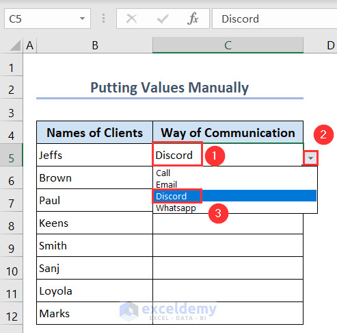
- Select any cell and press the Drop-Down button beside the cell, you’ll find the list. When you choose any item from the list, the item will be shown in the corresponding cell.
- If your worksheet is protected or shared, you can’t select the Data Validation option. So, unprotect the sheet or stop the sharing.
- The shortcut key for opening the Excel Data Validation dialog box is Alt + A + V + V.
- You can copy and paste the drop-down list by using keyboard shortcuts, Ctrl + C to copy and Ctrl + V to paste.
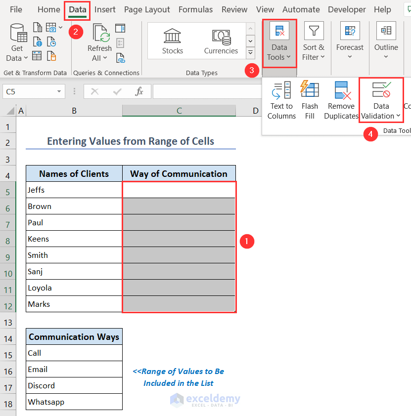
Method 2 – Insert List Values from a Range of Cells in Data Validation to Create a Drop-Down List
We’ll insert values from the range of cells B15:B18 to create a Drop-Down List.
- Select all the cells from C5:C12.
- Click on the Data Validation option under the Data Tools menu of the Data tab.
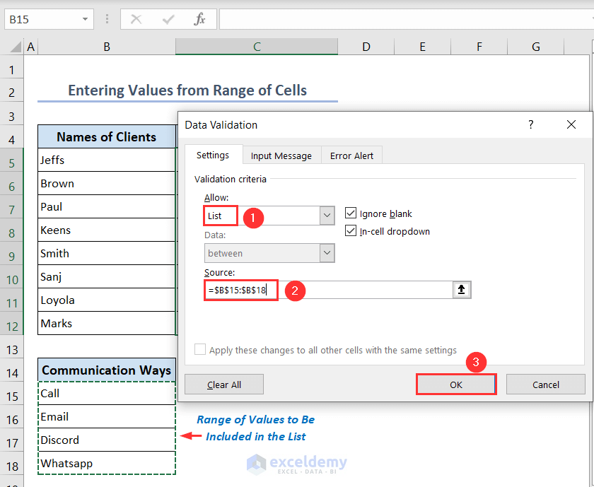
- In the Data Validation dialog box, select List under the Allow menu.
- In the Source box, put:
=$B$15:$B$18- Press the OK button.
- You can bring the range of values from other worksheets. For this, you have to include the sheet name in the Source box.
- Suppose the sheet name is Sheet1 from where you want to bring the values. Use this in the Source box: =Sheet1!$B$15:$B$18
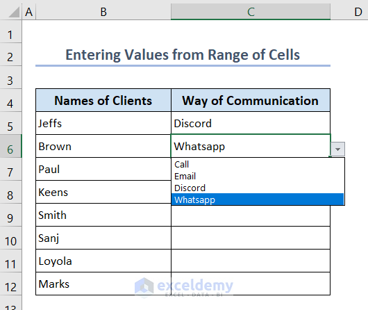
The list is ready to use.
- Include an empty cell from the bottom of the source range in the Data Validation dialog box. Your list will be dynamic as it will allow you to insert a blank option from the list.
- The advantage of this method is you can update your dropdown list by making changes in the given range. You don’t have to edit the Data Validation list.
- The disadvantage of this method is you need to update the Source range in the Data Validation dialog box to add or remove items from the list.
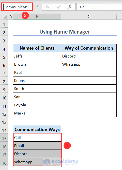
Method 3 – Apply the Name Manager in Data Validation to Make a Drop-Down List
- Select the cells B15:B18 and give them a name via the Name Box. We named them Communication.
- Open the Data Validation dialog box from the Data tab by selecting cells C5:C12.
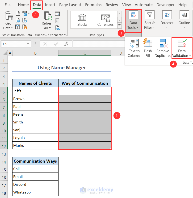
- Select List under the Allow menu and enter the range name in the Source box:
=Communication- Press the OK button.
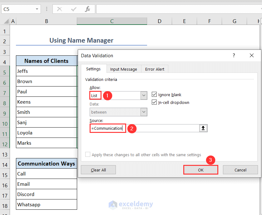
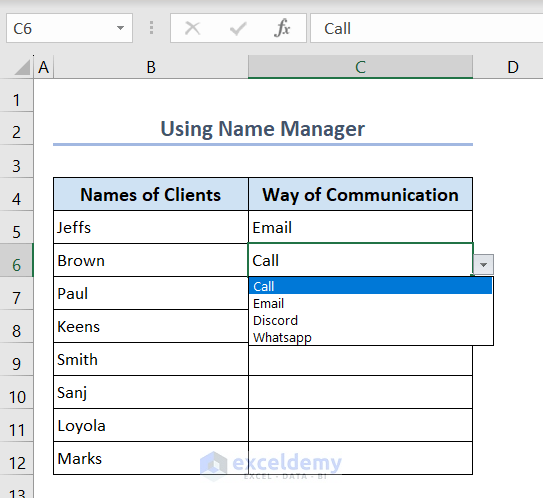
The list is now available.
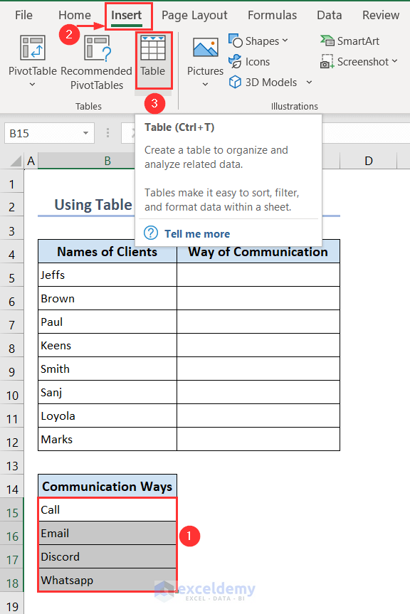
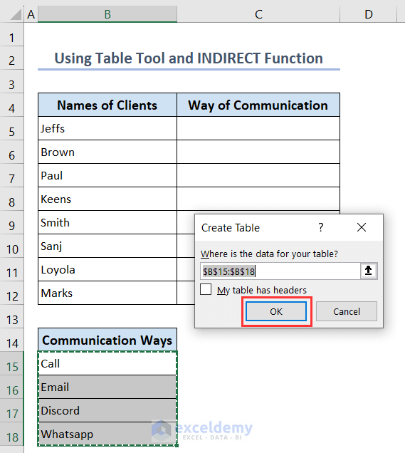
Method 4 – Combine the Table Tool and the INDIRECT Function in Data Validation
- To insert a Table, select the cells B15:B18 and click on the Table option from the Insert. Alternatively, press Ctrl + T.
- Press OK in the Create Table dialog box.
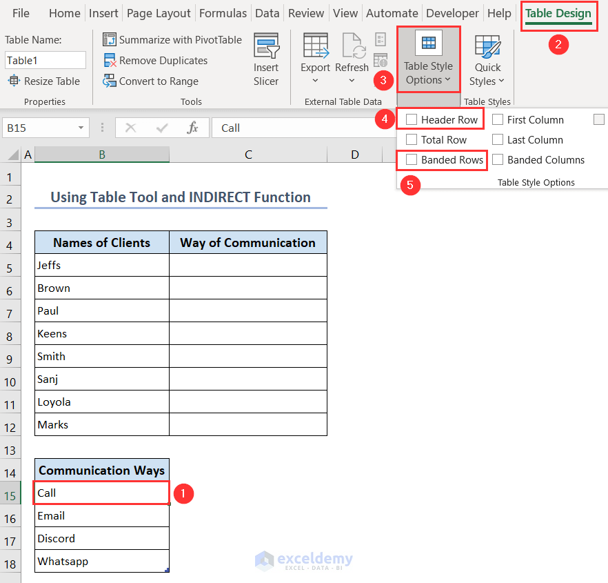
- Select any cell on the Table and go to the Table Design tab.
- Under the Table Style Options menu, untick the options Header Row and Banded Rows.
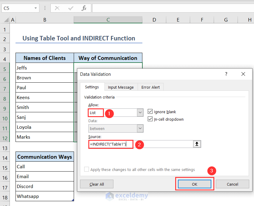
- Select cells C5:C12 and go to the Data Validation dialog box.

- Choose List from the Allow menu and use the following formula as the Source:
=INDIRECT("Table1")- Click the OK button.
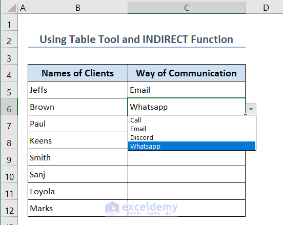
You’ll see the list of the values from the Table in your desired place.
Method 5 – Apply the OFFSET Function in Data Validation to Make a Drop-Down List
We want to make a drop-down list in cells C5:C12 with the items from cells B15:B18.
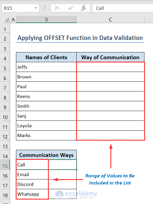
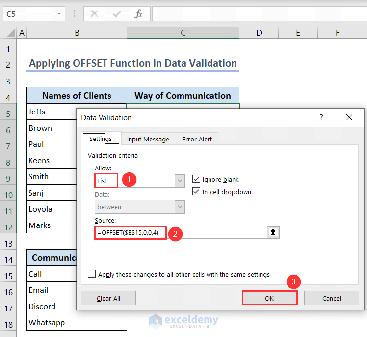
- Select all the cells from C5:C12 and go to the Data Validation dialog box.
- Choose List from the Allow menu and use the following formula as the Source:
=OFFSET($B$15,0,0,4)- Click the OK button.
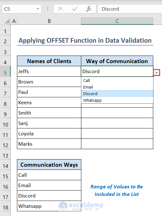
The drop-down list is ready.
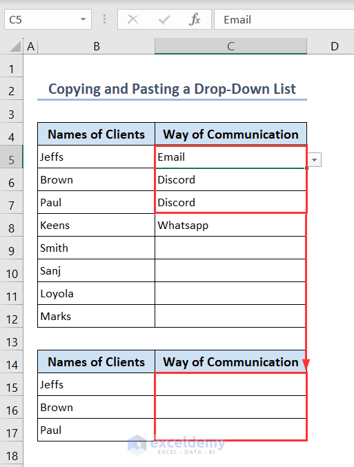
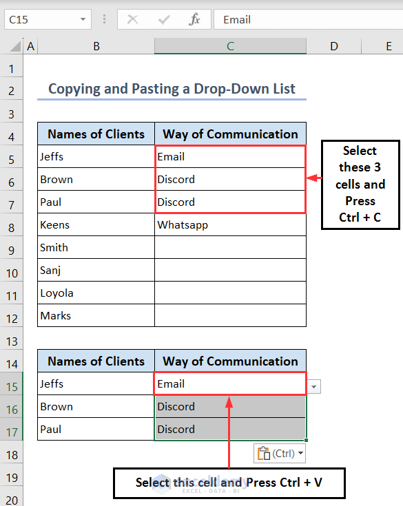
How to Copy and Paste a Drop-Down List to Other Cells in Excel
We want to copy the drop-down list in cells C5:C7 and paste it to cells C15:C17.
Method 1 – Copy and Paste Using Keyboard Shortcut
- Select cells C5:C7 and press Ctrl + C to copy the list.
- Select cell C15 and press Ctrl + V to paste the list.
Method 2 – Use the Paste Special Command
- Select cells C5:C7 and press Ctrl + C to copy the list.
- Select cell C15 and right-click.
- Click on the Paste Special option from the Context menu.
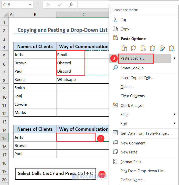
- The Paste Special dialog box will open.
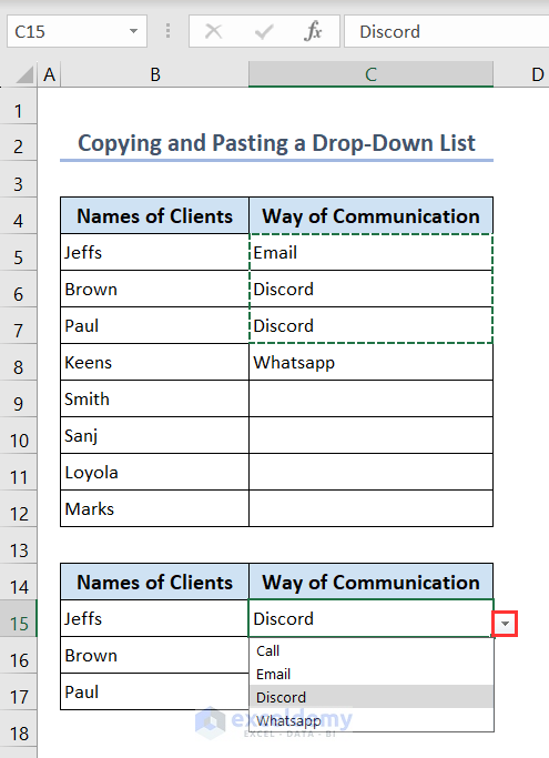
- Choose Validation and click OK.
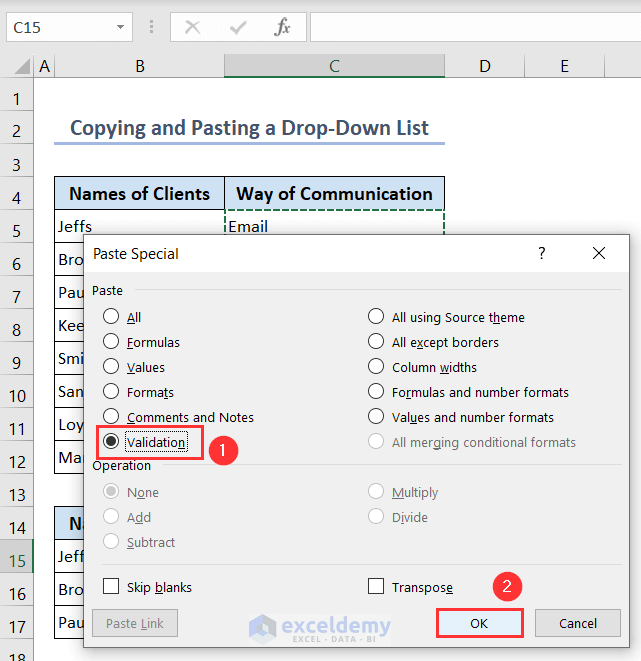
The drop-down list is pasted in cell C15.
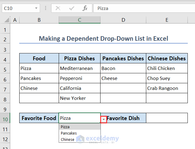
How to Make a Dependent Drop-Down List in Excel
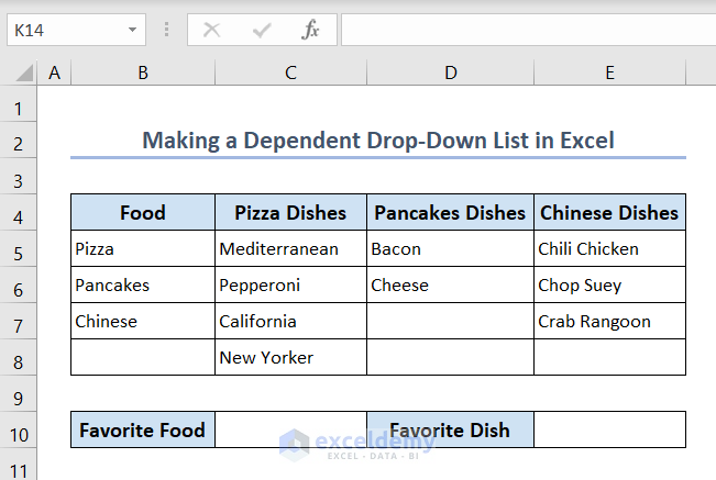
You can make a dependent drop-down list in Excel using the Name Manager and the INDIRECT function. We have a dataset having some food name and their different dishes. We want to make a list of food first. Then, we’ll make a dependent drop-down list of dishes based on the food items.
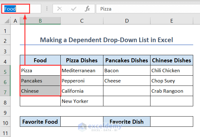
- Select all the cells B5:B7 and give them a name via Name Box. We named them Food.
- Name the other ranges: C5:C8 as Pizza, D5:D6 as Pancakes, and E5:E7 as Chinese.
- Select cell C10 and go to the Data Validation dialog box.
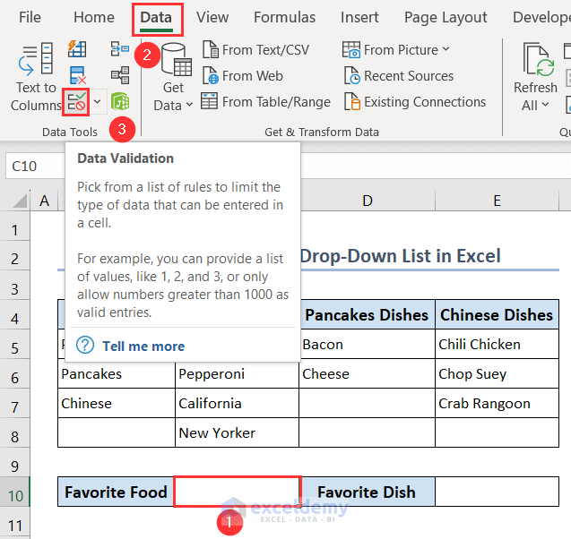
- Choose List from the Allow menu.
- Use the following formula as the Source:
=Food- Click the OK button.
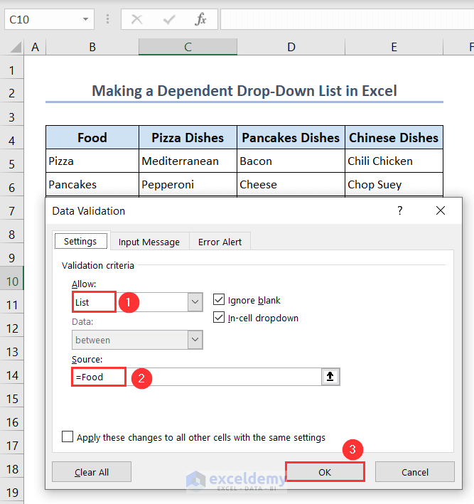
- The list of food is ready.
- Select cell E10 and go to the Data Validation dialog box.
- Choose List from the Allow menu.
- Use the following formula as the Source:
=INDIRECT($C$10)- Click the OK button.
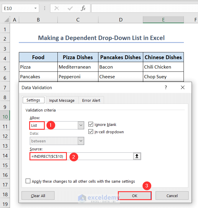
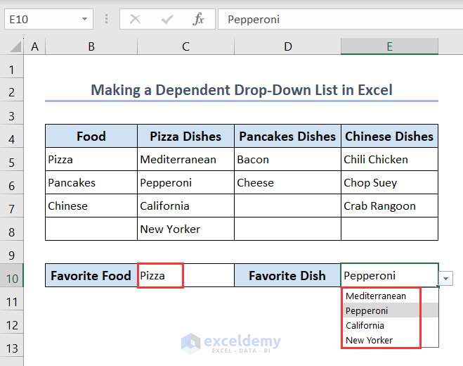
The dependent drop-down list is ready.
- Select Pizza from the first list. You’ll see only pizza-related dishes in the second list.
- If you change the parent drop-down after changing the dependent drop-down, the dependent drop-down will not change. So, it will be a wrong output.
- For example, if you select Pizza as the food and then select Pepperoni as the dish, and then go back and change the food to Pancakes, the dish would remain as Pepperoni.
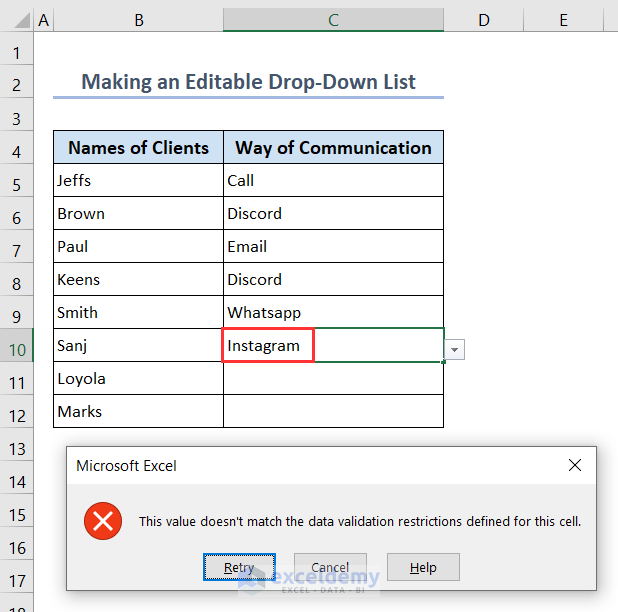
How to Make an Editable Drop-Down List in Excel
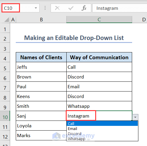
Whenever you make a Drop-Down list in Excel, it is uneditable. When we write the value Instagram in a cell, we get a warning message.
- Go to the Data Validation dialog box by selecting all cells from C5:C12.
- Go to the Error Alert tab and untick the option Show error alert after invalid data is entered.
- Press the OK button.
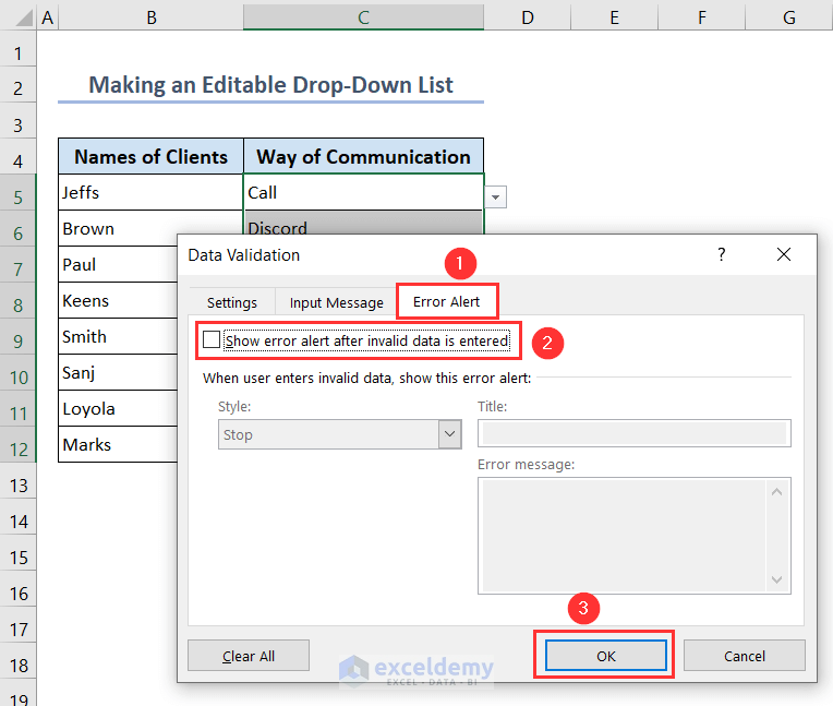
You can edit your list.
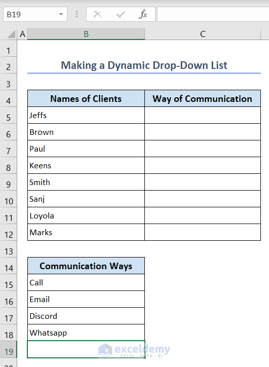
How to Make a Dynamic Drop-Down List in Excel
We want to make a drop-down list in cells C5:C12 with the items from cells B15:B19. We keep the cell B19 empty. We’ll put a new item in that cell to see if the list is dynamic or not.
Method 1 – Use the OFFSET and COUNTA Functions
- Select all the cells from C5:C12 and open the Data Validation dialog box.
- Choose List from the Allow menu and use the following formula as the Source:
=OFFSET($B$15, 0, 0, COUNTA($B:$B), 1)- Click the OK button.
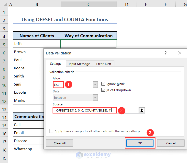
Formula Breakdown
- COUNTA($B:$B) – The COUNTA function counts the number of non-empty cells in column B.
- OFFSET($B$15, 0, 0, COUNTA($B:$B), 1)– The reference point for the offset is set to cell B15. By providing offsets of 0 rows and 0 columns, the range starts from the same row and column as the reference point. The height of the range is determined by the COUNTA function. Finally, the width of the range is set to 1 column.
To check whether it is dynamic or not, we add a new value Instagram in cell C19. The list gets updated automatically.
Method 2 – Use the OFFSET and COUNTIF Functions
- Select all the cells from C5:C12 and open the Data Validation dialog box.
- Choose List from the Allow menu and use the following formula as the Source:
=OFFSET($B$15, 0, 0, COUNTIF($B$15:$B$100,"<>"))- Click the OK button.
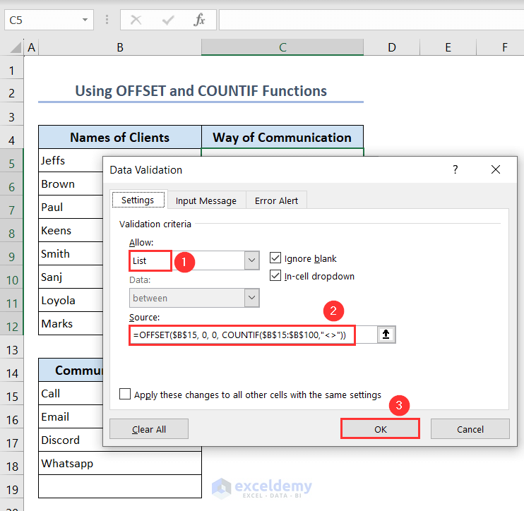
Formula Breakdown
- COUNTIF($B$15:$B$100,”<>”) – The COUNTIF function counts the number of non-empty cells in the range B15 to B100.
- OFFSET($B$15, 0, 0, COUNTIF($B$15:$B$100,”<>”)) – The reference point for the offset is set to cell B15. By providing offsets of 0 rows and 0 columns, the range starts from the same row and column as the reference point. The height of the range is determined by the COUNTIF function.
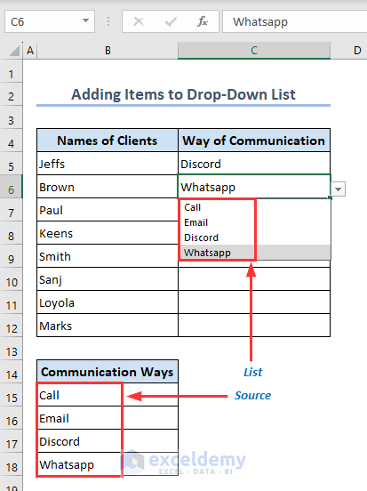
Add or Remove Items from a Drop-Down List without Opening Data Validation
Case 1 – Add Items to Drop-Down List Using Insert Command from Context Menu
We have a drop-down list. The source is from cells B15:B18.
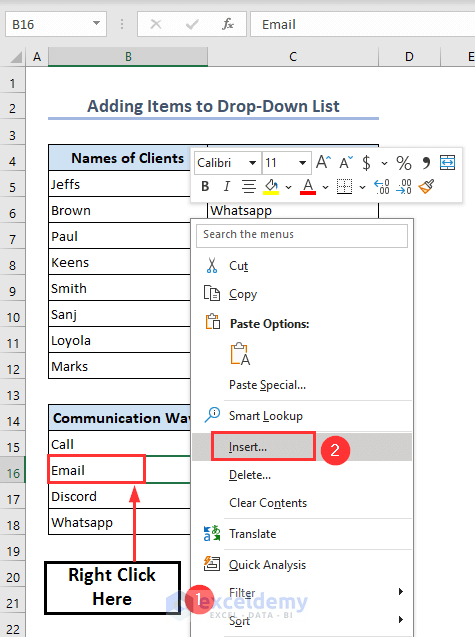
- Select cell B16 and right-click.
- Select the Insert option from the Context menu.
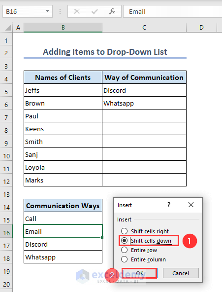
- Choose the option Shift cells down and press OK.
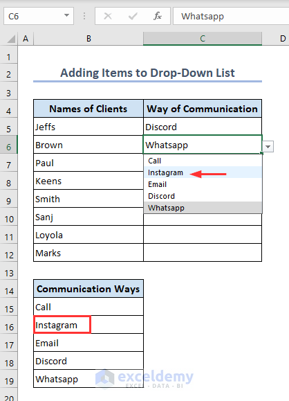
- Add Instagram in cell B16.
Case 2 – Remove Items from a Drop-Down List Using the Delete Command from Context Menu
- Select cell B16 and right-click.
- Select the Delete option from the Context menu.
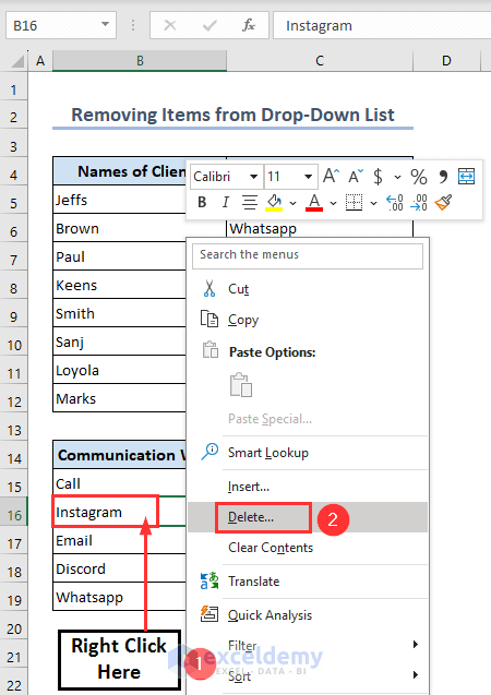
- Choose the option Shift cells up and press OK.
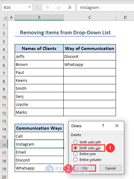
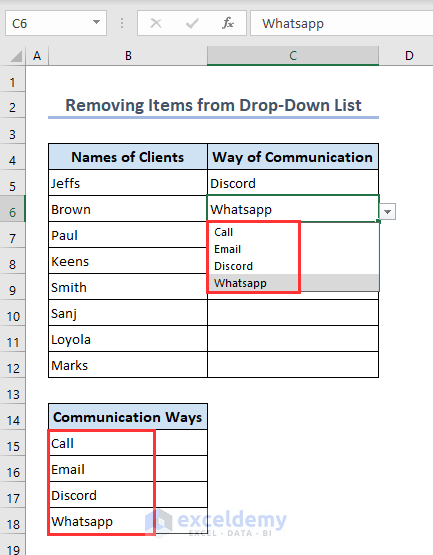
- This way, you can remove an item from the list.
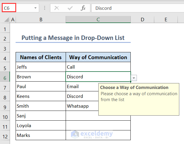
How to Input a Message in an Excel Drop-Down List
- Go to the Input Message tab of the Data Validation dialog box.
- Tick the option Show input message when cell is selected.
- Write the Title of the message and the message separately and press OK.
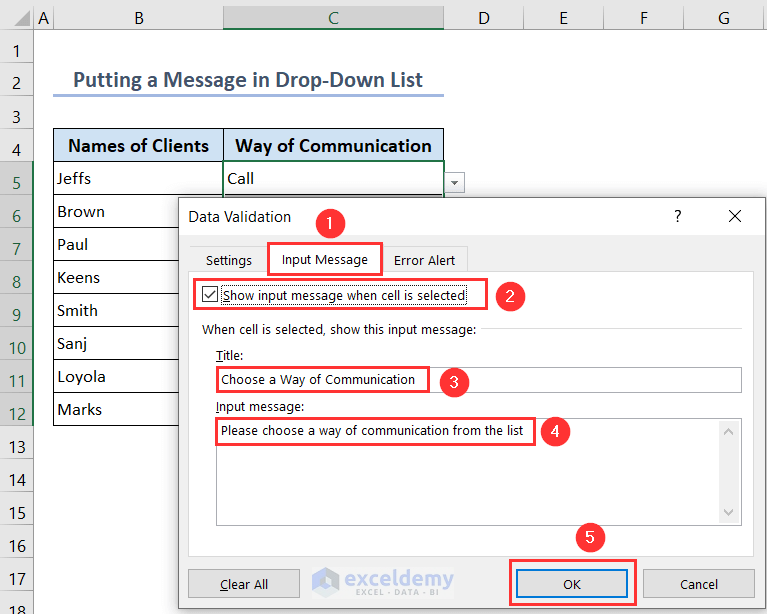
Whenever you select a cell in the list, you can see the corresponding message.
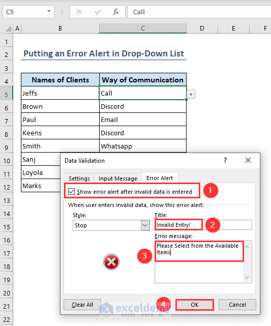
How to Put an Error Alert in an Excel Drop-Down List
- Open the Error Alert tab of the Data Validation dialog box.
- Tick the option Show error alert after invalid data is entered.
- Write the Title of the message and the message separately and press OK.
- We put the value Mobile in a cell and find an error alert.
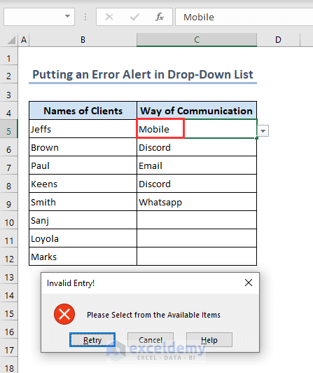
- We choose Stop from Style: box in the Error Alert tab of the Data Validation dialog box. This will stop anyone from editing the list.
- You can choose the Information or the Warning option from the Style: box. This will not stop anyone from editing the list.
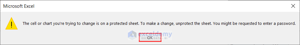
- We put a title and message on our own. The default title is “Microsoft Excel”. The default message is “The value you entered is not valid. A user has restricted values that can be entered into this cell”.
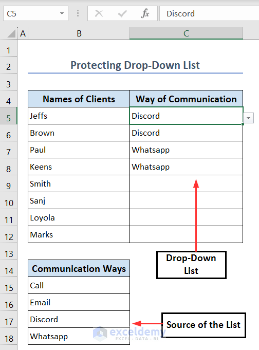
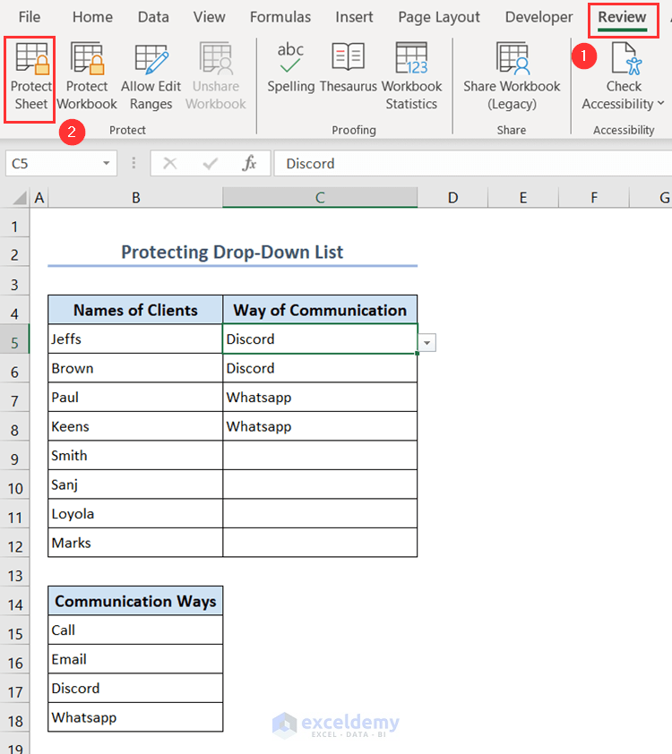
How to Protect Your Drop-Down List in Excel
We have the following drop-down list. The source range for this list is from cells B15:B18. Now, we’ll protect this drop-down list using the Protect Sheet option from the Review tab. After protecting sheet, no one can edit the drop-down list without unprotecting it.
- Go to Review tab and click the Protect Sheet option.
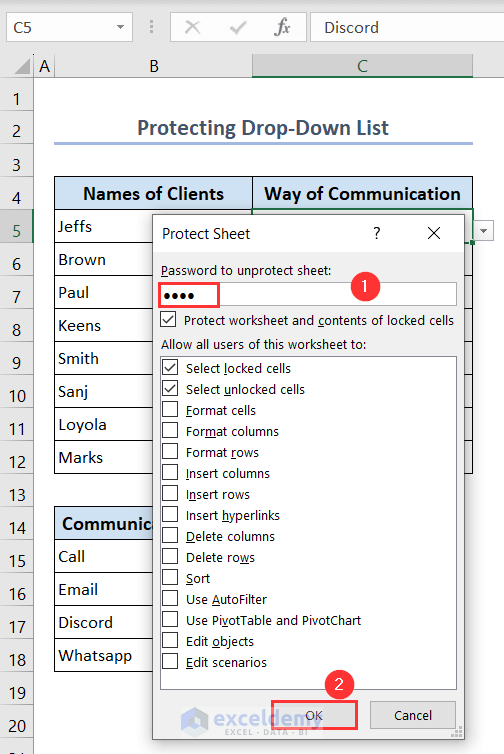
- The Protect Sheet dialog box will appear.
- Put a password. We put ‘list’.
- We can tick or untick any options but kept the defaults.
- Click OK.
- Put the same password and click OK.
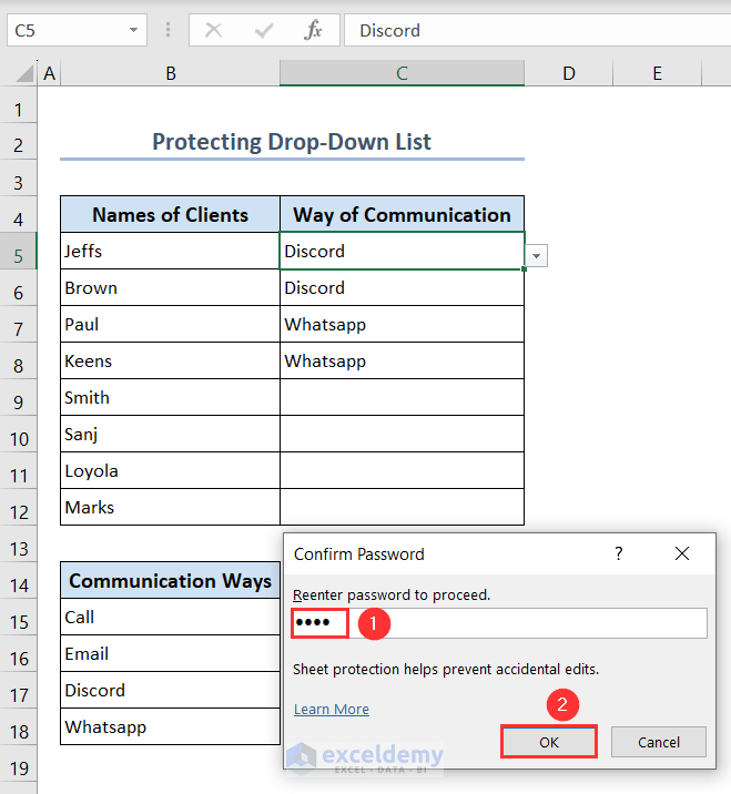
- The sheet is now protected.
- Let’s try to change Discord to Call in the list.
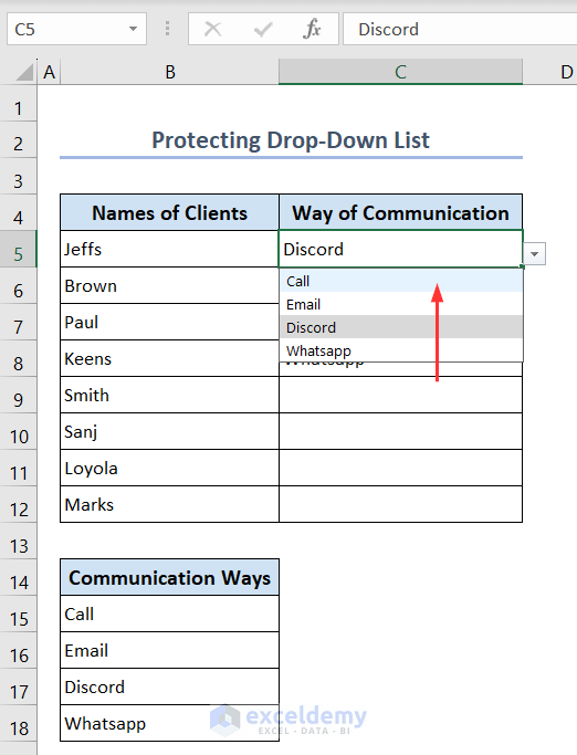
- The following warning message pops up. Click OK to close this.
How to Make a Custom List in Excel
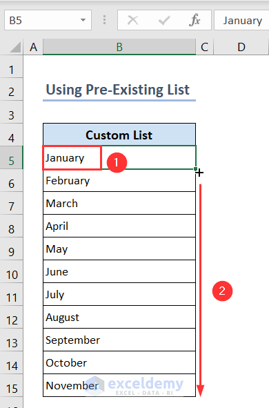
Method 1 – Use a Pre-Existing List
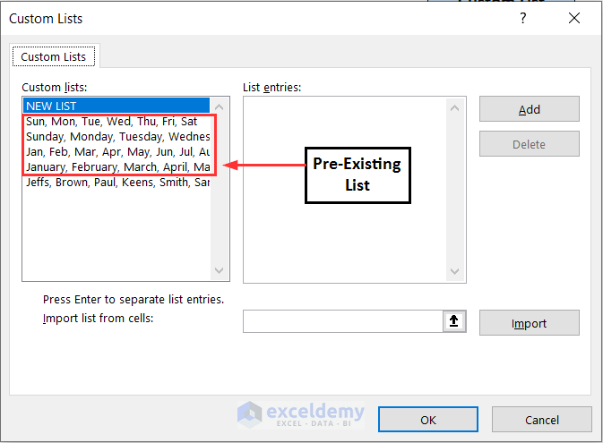
There are some pre-existing lists in Excel. We can find them by going to File >> Options >> Advanced >> General >> Edit Custom Lists.
- Put January in cell B5 and use the Fill Handle tool. You’ll get a custom list automatically.
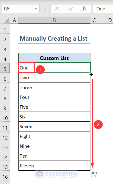
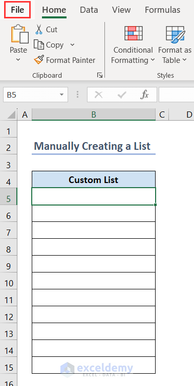
Method 2 – Manually Create a List as a Custom List
We will enter One in cell B5. We want to use the Fill Handle tool to create a list of numbers.
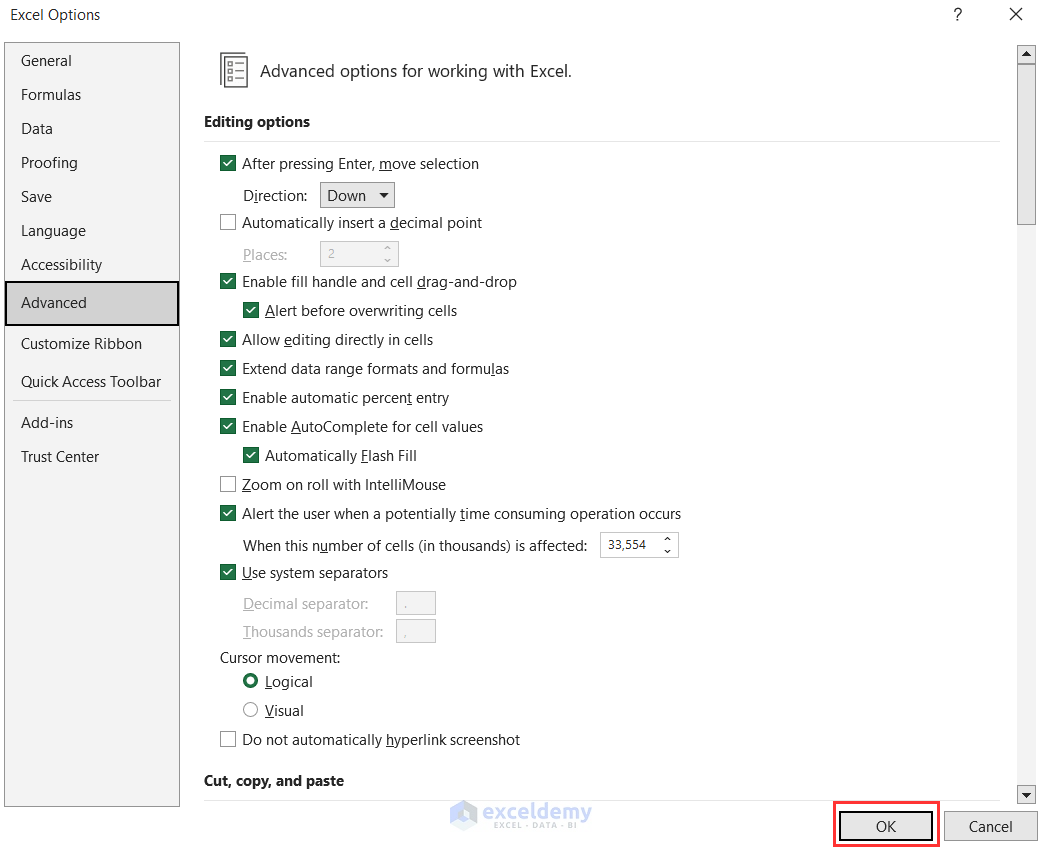
- Click on the File tab.
- Click on the Options menu.
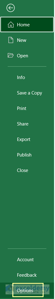
- In the Excel Options window, click on the Advanced menu.
- Click on the Edit Custom Lists button under the General section.
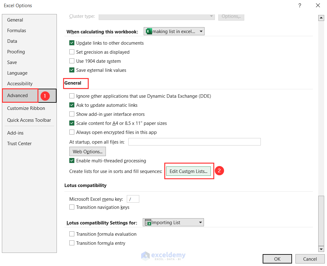
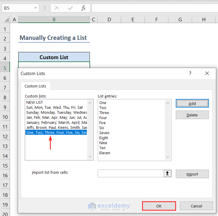
- The Custom Lists dialog box will open.
- Select NEW LIST option from the Custom lists: menu and type your list serially in the List entries: box, then click Add.
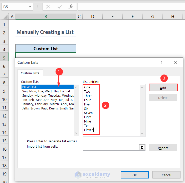
- The list will be added on the Custom lists: menu.
- Click OK.
- Click the OK button.
- Put One in cell B5 and use the Fill Handle tool. You’ll get the custom list.
How to Make a Unique List in Excel
We’ll use the SORT and UNIQUE functions to create a Unique List from the following names of clients.
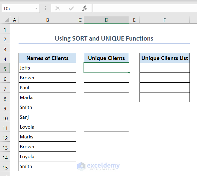
- Use the following formula in cell D5:
=SORT(UNIQUE(B5:B15))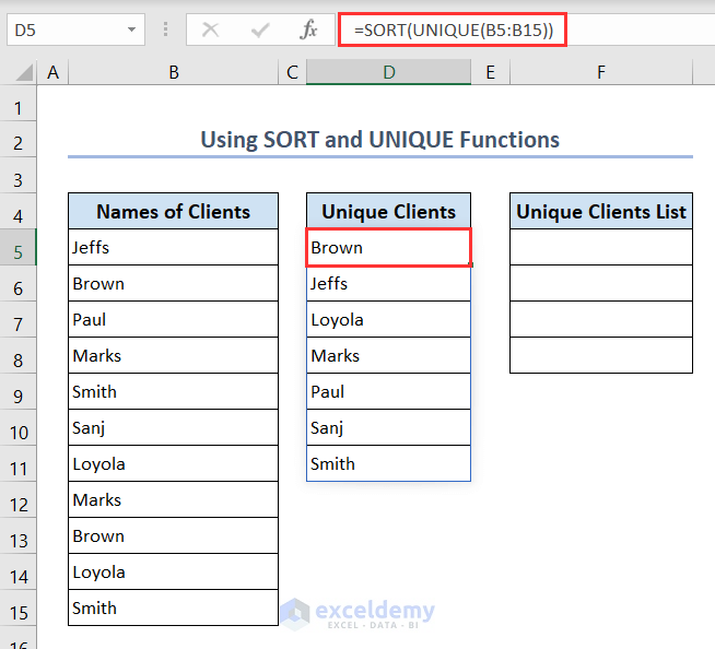
Formula Breakdown
- UNIQUE(B5:B15) – The UNIQUE function will get the unique values from the range B5:B15.
- SORT(UNIQUE(B5:B15)) – The SORT function then sorts the unique values.
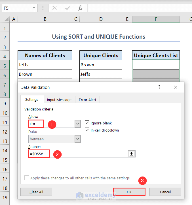
- Select all the cells from F5:F8 and go to Data Validation.
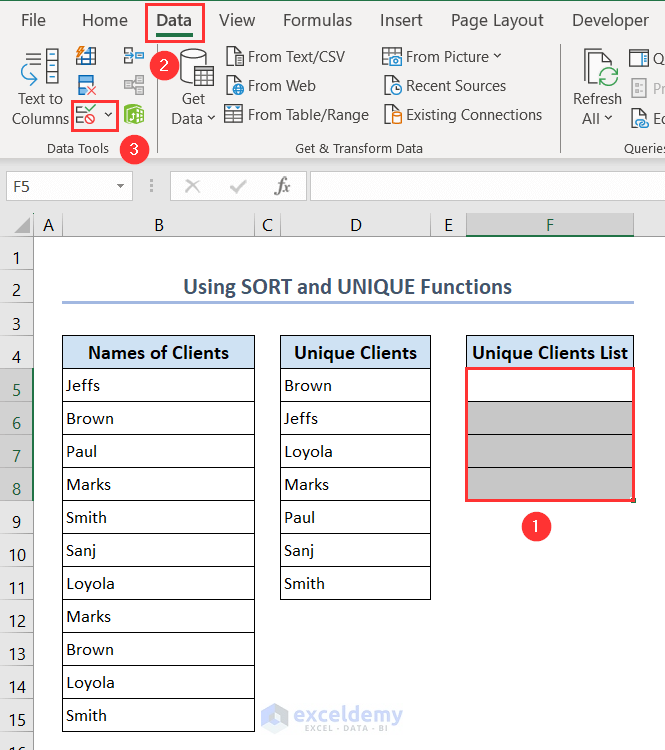
- In the Data Validation dialog box, select List under the Allow menu.
- In the Source box, use:
=$D$5#- Press the OK button.
The unique list is ready to use.
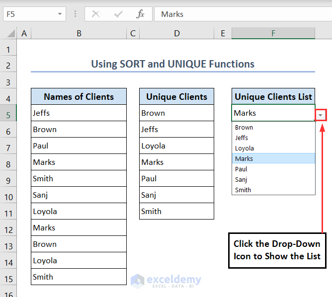
- The UNIQUE function will only be found in Microsoft 365 version.
- If you add new items, the UNIQUE function will automatically update the unique list and the drop-down list.
How to Import a List in Excel
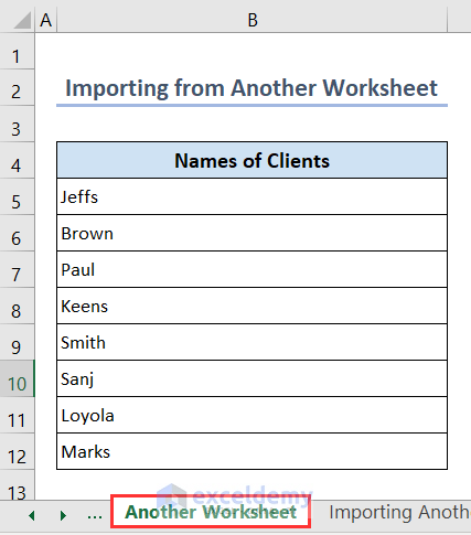
Case 1 – Import a Custom List from Another Worksheet
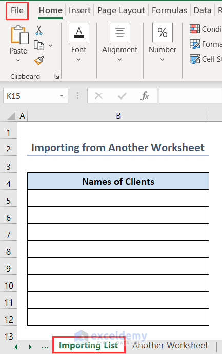
We have a list of client names on another sheet of the same workbook titled “Another Worksheet” and we want to import this custom list from this worksheet to our original worksheet.
- Go to the original worksheet titled “Importing List” and click on the File tab.
- Click on the Options menu.
- In the Excel Options window, click on the Advanced menu and click on the Edit Custom Lists button under the General section.
- Put the following cell reference in the box and press the Import button:
='Another Worksheet'!$B$5:$B$12- Click the OK button.
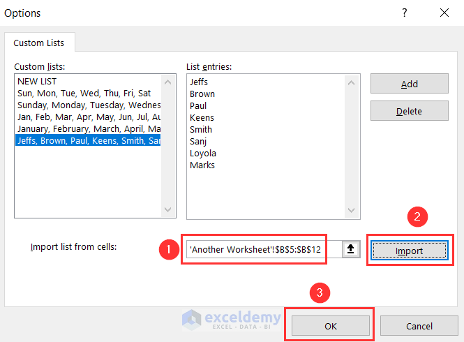
- Click the OK button.
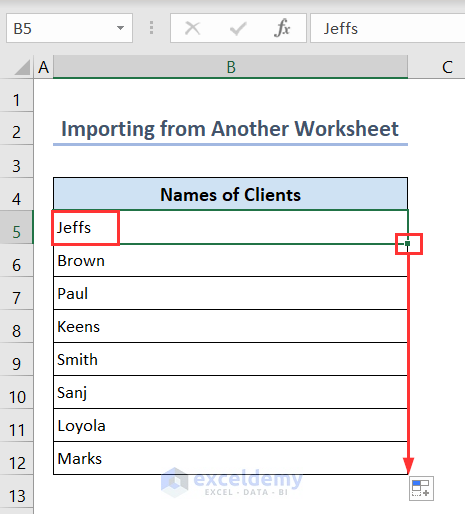
- When you type the first name Jeffs and drag the Fill Handle tool, you’ll get the full list of names automatically.
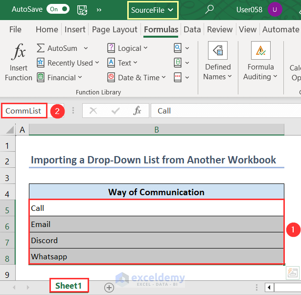
Case 2 – Import a Drop-Down List from Another Workbook
We have a list of communication methods in a different workbook titled “SourceFile”. We named it “CommList” using the Name Box feature. We’ll import this list into our original workbook.
- Go to Formulas and Define Name to open the Name Manager.
- In the New Name dialog box, give a name such as Items and type the following formula in the Refers to box and press OK.
=SourceFile.xlsx!CommList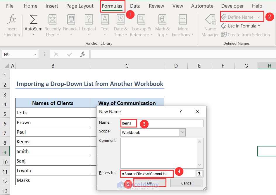
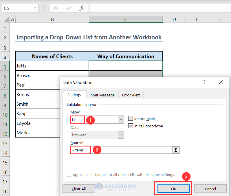
- Select cells C5:C12 and open the Data Validation dialog box.
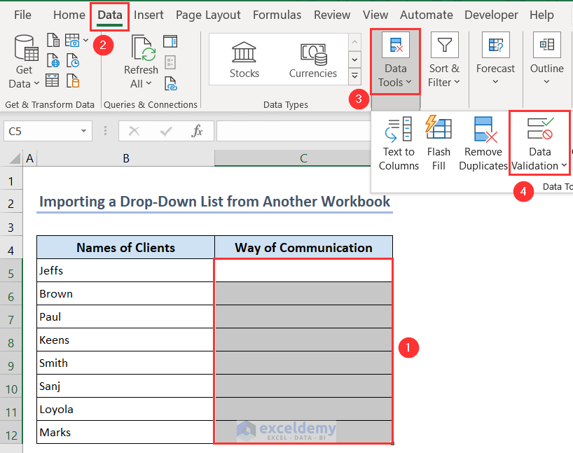
- Choose List from the Allow menu and use the following formula as the Source:
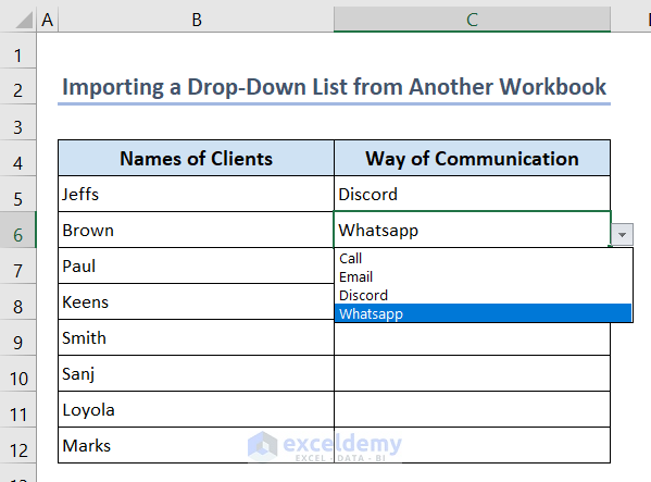
=Items- Click OK.
You’ll find the list where you want it.
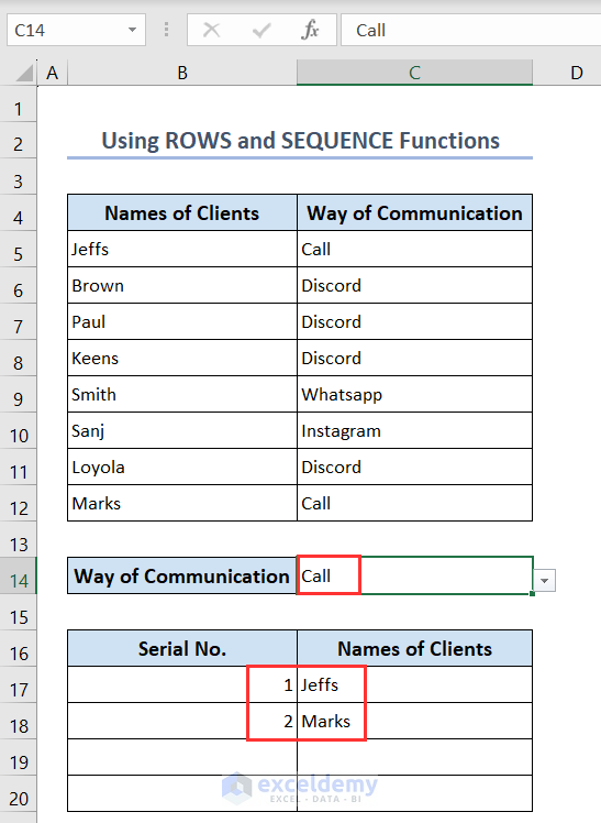
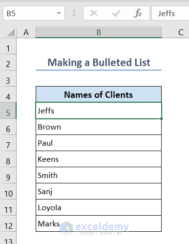
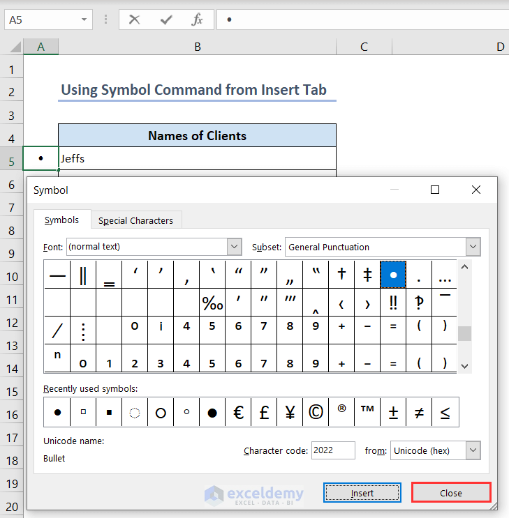
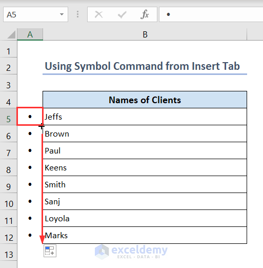
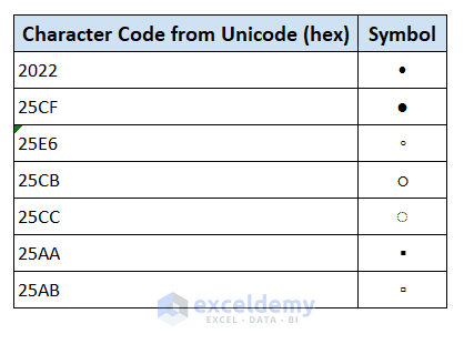
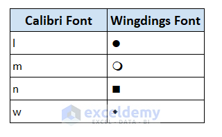
We have the same dataset as before. We’ll put a numbered list in cells B5:B12 which will be serial numbers of entries. The numbered list is ready. The numbered list is ready. The numbered list is ready. The numbered list is ready. The numbered list is ready. If you change the value in cell C14, you’ll see that the numbered list will update. We have a dataset with client names. We’ll make it a bulleted list. The bulleted list is ready. The bulleted list is ready. Here’s a list of character codes from Unicode (hex) and their symbols. You can use them in your list. The bulleted list is ready with the bullet inside the cell. The bulleted list is ready. The bulleted list is ready. Here’s a list of Calibri letters and their equivalent Wingdings symbols. You can use them in your list. After removing a list from your dataset, you can’t undo it. So, save the Excel file in another location before removing a list. You can make a list from 1 to 100 very easily in Excel. Just put the starting value in a cell and the second value in the cell after. Select the 2 cells and use the Fill Handle tool to drag. You’ll easily get a list from 1 to 100. Yes, you can make a random list in Excel by combining functions like SORTBY, RANDARRAY, and COUNTA functions. Let’s say you have a list of values in cells A1:A10. In another column (let’s say column B), enter the following formula in cell B1: You can make a list automatically in Excel using the SEQUENCE function. This function is only available in Microsoft 365. Suppose you want to make a list of numbers from 1 to 10. Just put the following formula in any cell: You can create a yes/no drop-down in Excel very easily. Select all the cells where you want to put the drop-down list. Go to Data > Data Tools > Data Validation. In the Data Validation dialog box, select List under the Allow menu. Write the values Yes and No manually separated by commas under the Source menu. Then press the OK button. No, you don’t need any formula to create drop-down lists in Excel. You have to use the Data Validation tool to create a drop-down list. No, a drop-down list is different from data filtering. We add a drop-down list to a cell or multiple cells in Excel to view a list of items. On the other hand, we add data filtering only to the headers of each column to filter data based on some categories. Download the Practice Workbook << Go Back to Excel Drop-Down List | Data Validation in Excel | Learn Excel
Note:
How to Make a Numbered List in Excel
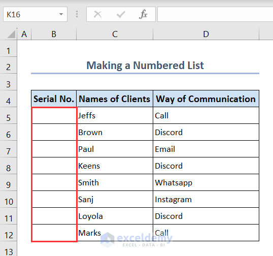
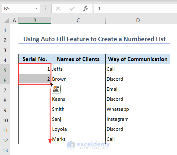
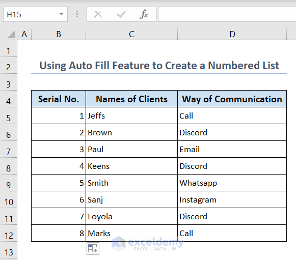
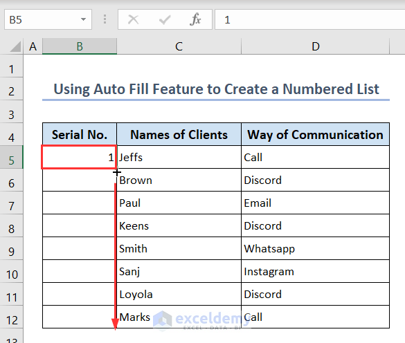
Method 1 – Use the AutoFill Feature to Create a Static Numbered List
Case 1.1 – Use the Fill Handle Tool
Case 1.2 – Use the Fill Series Option

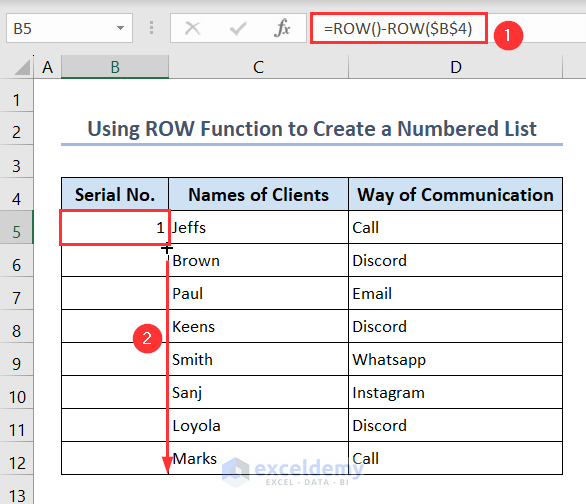
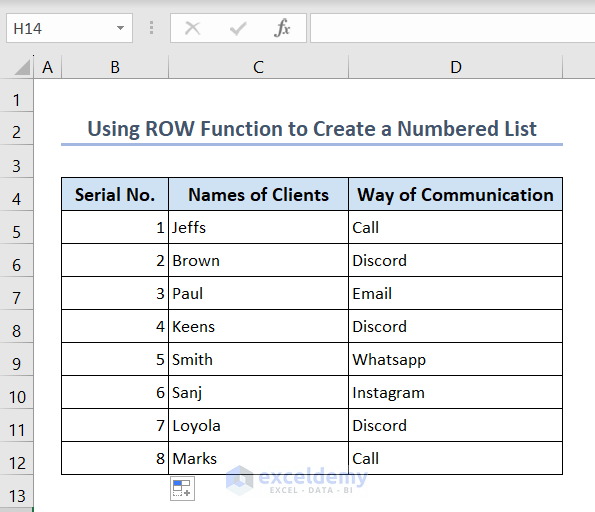
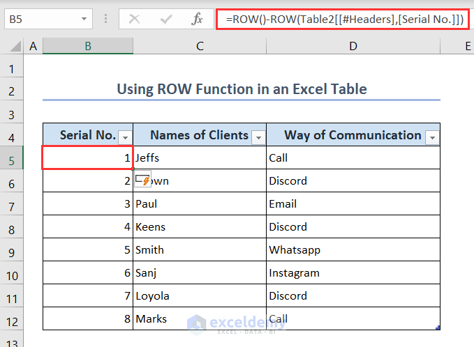
Method 2 – Use the ROW Function to Create a Numbered List
=ROW()-ROW($B$4)
Method 3 – Create a Dynamic Number List Using the ROW Function in an Excel Table
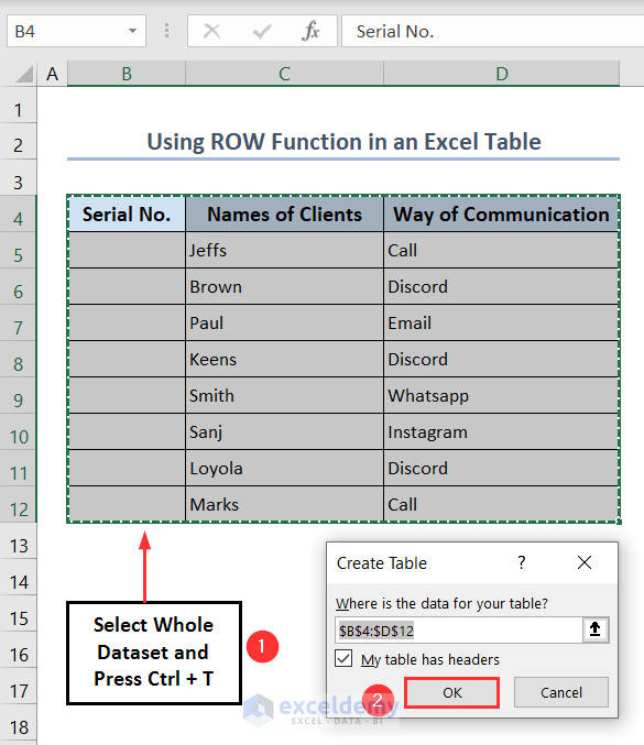
=ROW()-ROW(Table2[[#Headers],[Serial No.]])
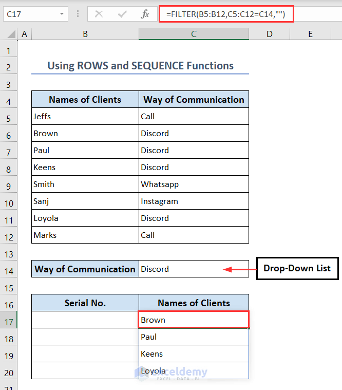
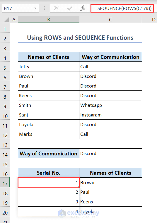
Method 4 – Make a Dynamic Numbered List Using ROWS and SEQUENCE Functions
=FILTER(B5:B12,C5:C12=C14,"")
=SEQUENCE(ROWS(C17#))
How to Make a Bulleted List in Excel
Method 1 – Use Keyboard Shortcuts to Add Bullet Points
Method 2 – Use the Symbol Command to Add Bullet Points in Other Cells
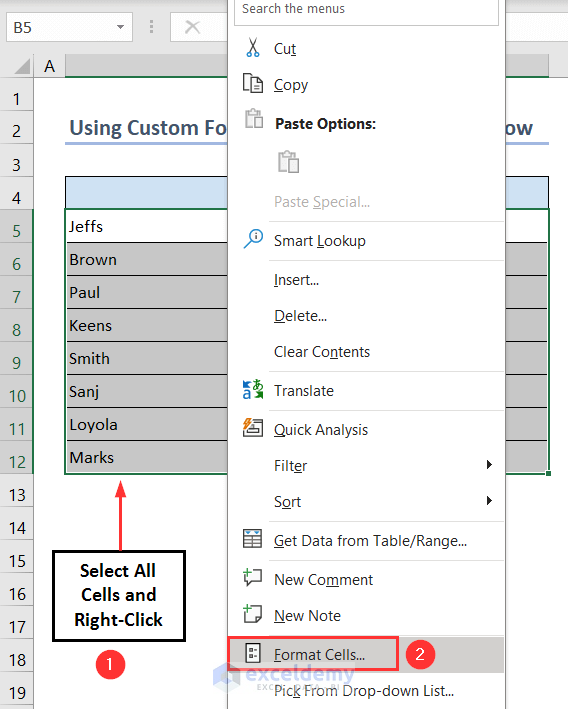
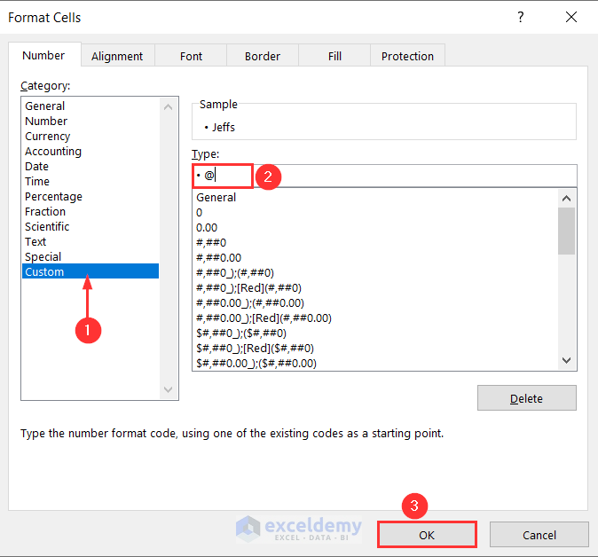
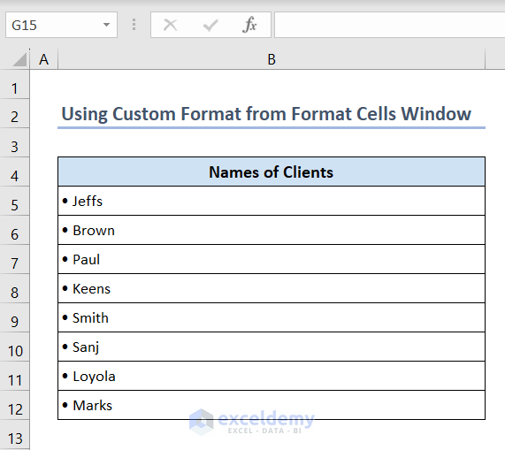
Method 3 – Use the Custom Format to Add Bullet Points in the Same Cell
• @
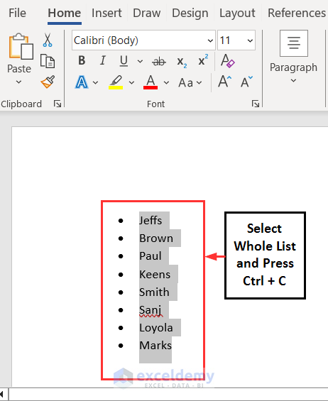
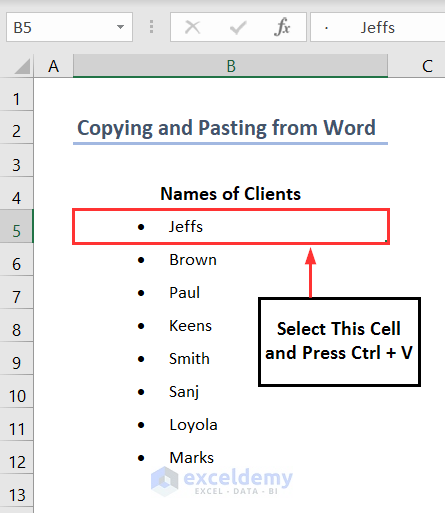
Method 4 – Create a Bulleted List by Copying and Pasting from Word
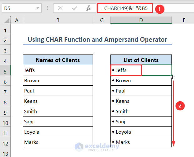
Method 5 – Use the CHAR Function and the Ampersand Operator
=CHAR(149)&" "&B5
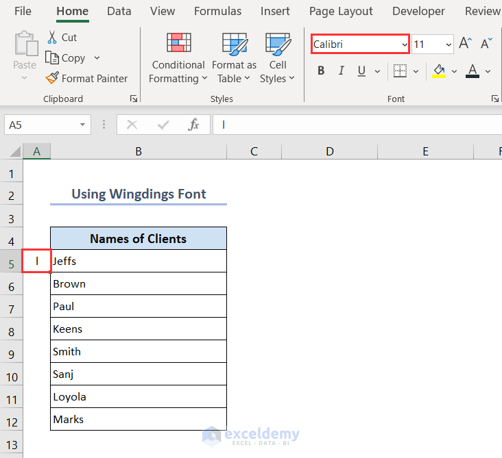
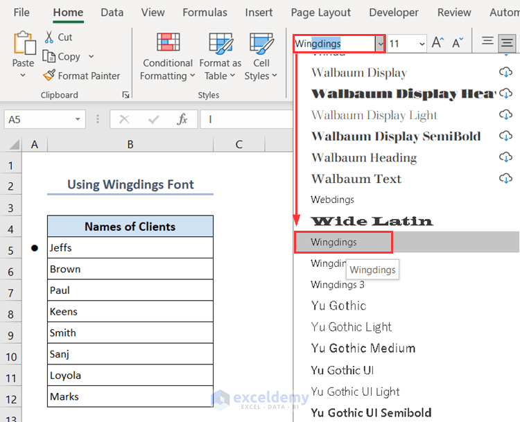
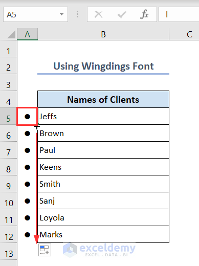
Method 6 – Use the Wingdings Font to Add Bullet Points
How to Remove a List from Excel
Things to Remember
Frequently Asked Questions
How do I make a list from 1 to 100 in Excel
Can Excel make a random list?
=SORTBY(A1:A10,RANDARRAY(COUNTA(A1:A10)))
You will have a random list of values in column B.How do I make a list automatically in Excel?
=SEQUENCE(10)
You will have a random list of numbers from 1 to 10.How do I create a yes/no drop-down in Excel?
Do I need a formula to create drop-down lists?
Is a drop-down list the same as data filtering?
Make List in Excel: Knowledge Hub

