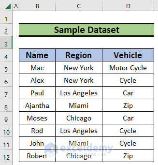
How to Generate List Based on Criteria in Excel (5 Methods)

We have a dataset of several people from different locations along with their vehicles. Using this data, we will form a list based on criteria.

excel generate list based on criteria

Method 1 – Using the INDEX-SMALL Combination to Generate a List

Steps:

Select the F5 cell and insert:

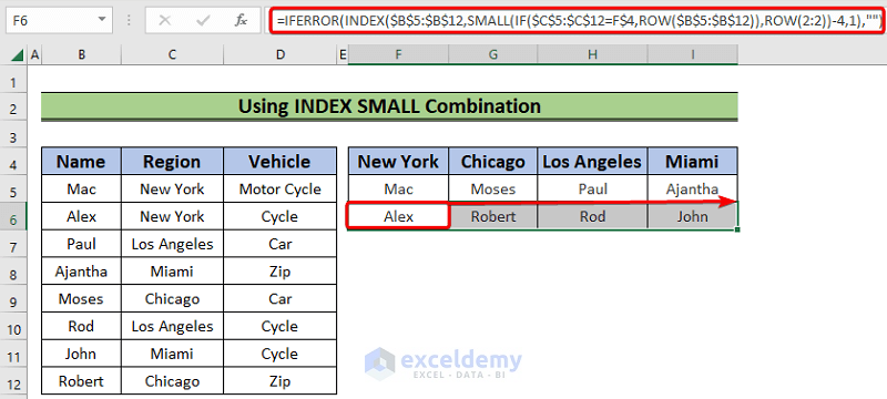
=IFERROR(INDEX($B$5:$B$12,SMALL(IF($C$5:$C$12=F$4,ROW($B$5:$B$12)),ROW(1:1))-4,1),"")

Press Enter.

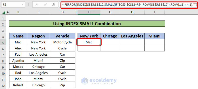
wrting formula to generate list based on criteria excel

We will get the name associated with the region.
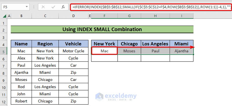
AutoFill the values to the right for the rest of the regions.

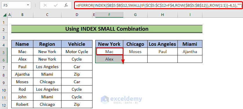
autofill formula to generate list based on criteria excel

Drag the Fill Handle down from the F5 cell.

Drag the Fill Handle to the right to AutoFill the values for the rest of the regions.

Formula Breakdown

IF($C$5:$C$12=F$4,ROW($B$5:$B$12)): The ROW($B$5:$B$12) returns an array of values of rows, {5;6;7;8;9;10;11;12}. Again, $C$5:$C$12=F$4 expression returns an array of TRUE and FALSE the {TRUE;TRUE;FALSE;FALSE;FALSE;FALSE;FALSE;FALSE}. So, finally the IF function returns the values from the {5;6;7;8;9;10;11;12} array which matches the TRUE values from the {TRUE;TRUE;FALSE;FALSE;FALSE;FALSE;FALSE;FALSE} array and keeps the rest of the values FALSE.
- Output : {5;6;FALSE;FALSE;FALSE;FALSE;FALSE;FALSE}.
SMALL({5;6;FALSE;FALSE;FALSE;FALSE;FALSE;FALSE},ROW(1:1)): It becomes SMALL({5;6;FALSE;FALSE;FALSE;FALSE;FALSE;FALSE},{1}). The SMALL function returns the 1st smallest value from the {5;6;FALSE;FALSE;FALSE;FALSE;FALSE;FALSE} array. So, the output will be {5}.
- Output: {5}.
INDEX($B$5:$B$12,{5}-4,1): The INDEX($B$5:$B$12,{5}-4,1) becomes INDEX($B$5:$B$12,1,1). The INDEX function will return the first value in the $B$5:$B$12 range which is Mac.
- Output: “Mac”
IFERROR(INDEX($B$5:$B$12,SMALL(IF($C$5:$C$12=F$4,ROW($B$5:$B$12)),ROW(1:1))-4,1),””): The entire formula becomes IFERROR(“Mac”,””). The IFERROR function will return Mac.
- Output: Mac

Method 2 – Using the AGGREGATE Function to Generate a List

Steps:

Choose the F5 cell and insert:

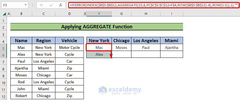
=IFERROR(INDEX($B$5:$B$12,AGGREGATE(15,6,IF($C$5:$C$12=F$4,ROW($B$5:$B$12)-4),ROW(1:1)),1),"")

Hit Enter.

using the aggregate function to generate list based on criteria excel

AutoFill the values for the remaining regions.

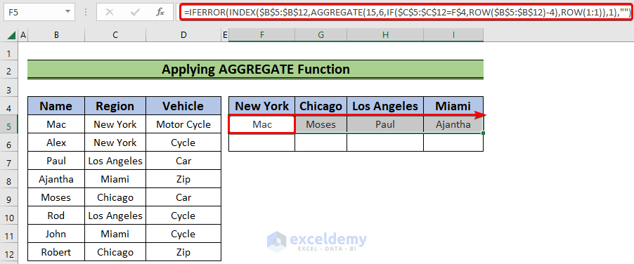
You can drag the fill handle down to get the next values.

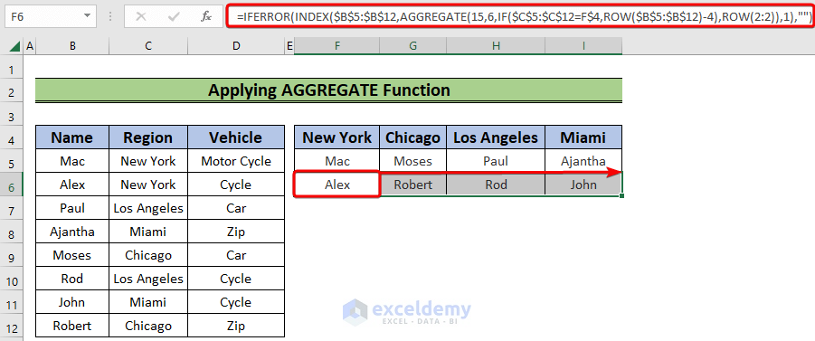
Drag to the right to AutoFill the values for the rest of the regions.

Formula Breakdown

IF($C$5:$C$12=F$4,ROW($B$5:$B$12)-4): The formula becomes IF({TRUE;TRUE;FALSE;FALSE;FALSE;FALSE;FALSE;FALSE},{5;6;7;8;9;10;11;12}). After deducting 4 from each values of {5;6;7;8;9;10;11;12} the set becomes {1;2;3;4;5;6;7;8}. Finally, the IF function will return {1;2;FALSE;FALSE;FALSE;FALSE;FALSE;FALSE}.
- Output: {1;2;FALSE;FALSE;FALSE;FALSE;FALSE;FALSE}
AGGREGATE(15,6,IF($C$5:$C$12=F$4,ROW($B$5:$B$12)-4),ROW(1:1)): The number 15 in the AGGREGATE denotes the SMALL function. So the expression becomes SMALL({1;2;FALSE;FALSE;FALSE;FALSE;FALSE;FALSE},{1}). And the expression will return {1}.
- Output: {1}
INDEX($B$5:$B$12,AGGREGATE(15,6,IF($C$5:$C$12=F$4,ROW($B$5:$B$12)-4),ROW(1:1)),1): It will become INDEX($B$5:$B$12,{1},1). The INDEX function will return the first value of the $B$5:$B$12 range which is Mac.
- Output: “Mac”
IFERROR(INDEX($B$5:$B$12,AGGREGATE(15,6,IF($C$5:$C$12=F$4,ROW($B$5:$B$12)-4),ROW(1:1)),1),””): Finally, this expression will become IFERROR(“Mac”,””). Thus the IFERROR function will return Mac.
- Output: Mac

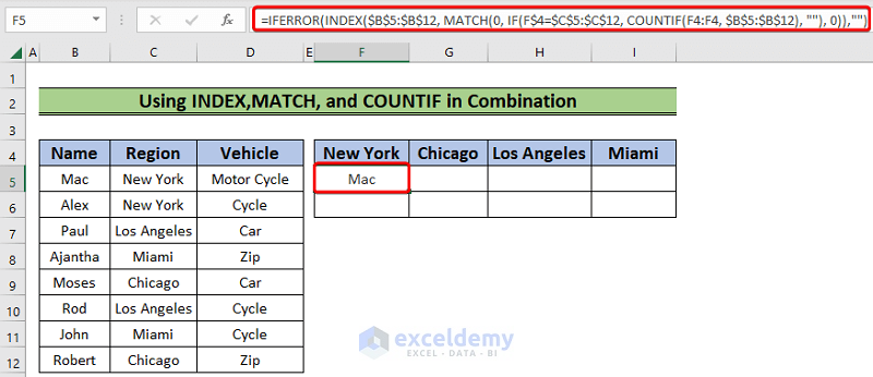
Method 3 – Generate Unique List Using INDEX-MATCH-COUNTIF

Steps:

Select the F5 cell and insert the following:

=IFERROR(INDEX($B$5:$B$12, MATCH(0, IF(F$4=$C$5:$C$12, COUNTIF(F5:F5, $B$5:$B$12), ""), 0)),"")

Press the Enter button.

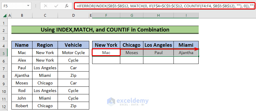
using index, match and countif functions to generate list based on criteria excel

Drag the Fill Handle to the right to AutoFill the values.

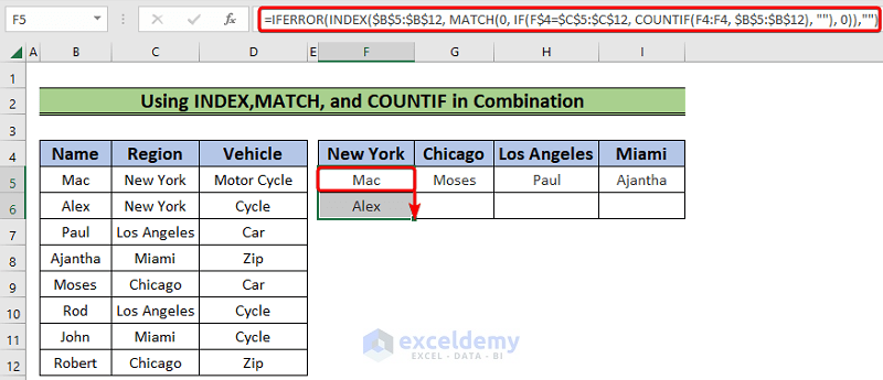
Drag the Fill Handle down from the F5 cell to AutoFill for New York.

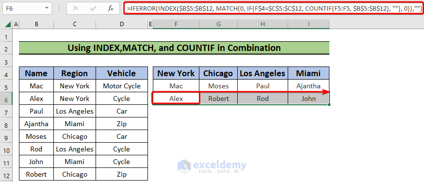
autofill formula to generate list based on criteria excel

Drag the Fill Handle to the right to AutoFill the values for the remaining regions.

Formula Breakdown

COUNTIF(F4:F4, $B$5:$B$12): The expression becomes {0;0;0;0;0;0;0;0}. As the COUNTIF function can not find any of the values in the $B$5:$B$12 range from the F4:F4.
- Output: {0;0;0;0;0;0;0;0}
IF(F$4=$C$5:$C$12, COUNTIF(F4:F4, $B$5:$B$12), “”): The expression becomes {0;0;””;””;””;””;””;””}. As the F$4=$C$5:$C$12 returns an array like this- {TRUE;TRUE;FALSE;FALSE;FALSE;FALSE;FALSE;FALSE}.
- Output: {0;0;””;””;””;””;””;””}.
MATCH(0, IF(F$4=$C$5:$C$12, COUNTIF(F4:F4, $B$5:$B$12)): This expression becomes MATCH(0, {0;0;””;””;””;””;””;””}). The MATCH function matches 0 with the first value of the {0;0;””;””;””;””;””;””} set and will return 1.
- Output: 1
INDEX($B$5:$B$12, MATCH(0, IF(F$4=$C$5:$C$12, COUNTIF(F4:F4, $B$5:$B$12), “”), 0)): The expressioin will become INDEX($B$5:$B$12,1). The INDEX function will return the first value of the $B$5:$B$12 range that is Mac.
- Output: “Mac”.
IFERROR(INDEX($B$5:$B$12, MATCH(0, IF(F$4=$C$5:$C$12, COUNTIF(F4:F4, $B$5:$B$12), “”), 0)),””): This expression becomes IFERROR(“Mac”,””). So, the IFERROR function will return Mac.
- Output: Mac

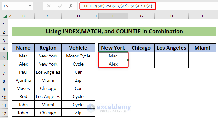
Method 4 – Using the FILTER Function to Generate a List Based on Criteria

Only works on Excel 365.

Steps:

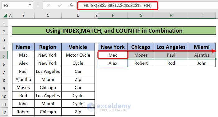
Choose the F5 cell and enter the following:

=FILTER($B$5:$B$12,$C$5:$C$12=F$4)

Hit the Enter button.

using filter function to generate list based on criteria excel

AutoFill the values for the rest of the regions.

Method 5 – Applying the TEXTJOIN Function

Steps:

Select the G5 cell and enter the following:

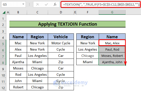
=TEXTJOIN(", ",TRUE,IF(F5=$C$5:C12,$B$5:$B$12,""))

Press Enter.

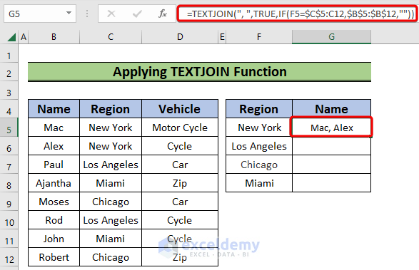
applying textjoin function to generate list based on criteria excel

We will get the names for that particular region separated by comma.
Drag the AutoFill down to AutoFill the values.

Download the Practice Workbook

Generate List Based on Criteria.xlsx

Further Readings

<< Go Back to Make List in Excel | Excel Drop-Down List | Data Validation in Excel | Learn Excel

Get FREE Advanced Excel Exercises with Solutions!

27 Comments

Ken S Jan 7, 2022 at 9:04 PM

Not a single one of these formulas work. I have used them all in the practice workbook, outlined exactly as you present and none of them work.
- Reply
  Kawser Jan 7, 2022 at 11:15 PM
  
  Did you download the working file? We use Microsoft 365 for making our Excel tutorials. Please download the workbook and let me know whether the system works or not.
  Thanks.
Ling Feb 4, 2022 at 7:20 PM

For this formula, =IFERROR(INDEX($B$2:$B$12, MATCH(0, IF(G$2=$C$2:$C$12, COUNTIF($G$2:$G2, $B$2:$B$12), “”), 0)),””) is it possible to create the list based on multiple criteria? Eg, names by region based on Motor Vehicles
- Reply
  Naimul Hasan Arif Aug 17, 2022 at 12:16 PM
  
  Thanks for your query.
  Yes, it is possible to apply multiple criteria. Not sure how your data looks, but according to your query, I have tried to reorganize it as follows to categorize names by region based on Vehicle.
  
  =INDEX(B5:B15,MATCH(1,(B18=$D$5:$D$15) * (C18=$C$5:$C$15),0))
rick Apr 14, 2022 at 4:26 PM

Is it possible to put all the names in one cell?
- Reply
  Naimul Hasan Arif Aug 17, 2022 at 3:02 PM
  
  Definitely possible. You just need to concatenate the values in a cell, can use the TEXTJOIN function to do so.
  
  I have the use the following formula for this case.
  
  =TEXTJOIN(“, “,TRUE,IF(F5=$C$5:$C$15,$B$5:$B$15,””))
Philip Jun 14, 2022 at 9:07 PM

Wow. Very handy. And very nicely done! kudos
- Reply
  Naimul Hasan Arif Aug 21, 2022 at 12:01 PM
  
  Thanks for your appreciation. It means a lot.
- Reply
  Bella Jul 22, 2022 at 8:53 AM
  
  Can I use this if I want to search row 23 for the value “2” in order to obtain the information from Row 6? I would want it to provide a list just as it is above too so no repeat values.
Just Jul 15, 2022 at 11:43 PM

How do you modify the formula if your ranges does not start on row 1?
For example your data start at row 6. Then none of the formulas is working properly.
- Reply
  Naimul Hasan Arif Aug 17, 2022 at 5:48 PM
  
  Unfortunately for some strange reasons, the formulas with the INDEX function don’t behave properly while starting from any other row but row 1. But luckily you have some other alternatives like the FILTER function in case your dataset start from row6
Bella Jul 22, 2022 at 8:56 AM

Can you modify the formula for a row search. The value I am searching for is “2” in row 23. The value I want returned is in Row 6. I would want it to create a list just as displayed above each time a 2 is found in row 23 of the values in row 6. Is this possible?
- Reply
  Naimul Hasan Arif Aug 21, 2022 at 12:05 PM
  
  You can apply the INDEX – MATCH functions combination to find out whether the value is matching with “2 ” or not in row 23 and then, use the INDIRECT function to retrieve the matched value with the value in row 6.
Rav Nov 11, 2022 at 12:54 AM

Hi,

When I reference criteria from another worksheet, it generates an error – any thoughts?
- Reply
  Shahriar Nov 13, 2022 at 4:08 PM
  
  Hi RAV,
  It would be great if you share your Excel workbook. Because this formula works fine with criteria from other worksheets in our workbook.
  See the screenshot below.
  
  In Sheet3, we inserted the formula and gave all the arguments from Sheet2.
  =IFERROR(INDEX('INDEX - SMALL Formula'!$B$2:$B$12,SMALL(IF('INDEX - SMALL Formula'!$C$2:$C$12=G$4,ROW('INDEX - SMALL Formula'!$B$2:$B$12)-1),ROW('INDEX - SMALL Formula'!1:1)),1),"")
  And, it’s working without any errors. So, there must be another problem with your workbook. So, please share it with us thus we can solve your issue.
  If there is any other problem regarding Excel, you can let us know. Also, follow our website, ExcelDemy, a one-stop Excel solution provider to explore more. Happy Excelling.
anil bhatia Mar 4, 2023 at 2:27 PM

it is not working for me i tried using
=IFERROR(INDEX($B$5:$B$10,SMALL(IF(F$4=$C$5:$C$10,ROW($B$5:$B$10)),ROW(1:1))-4,1),”NA”)
but it shows only first value and not beyond
Values in Col B
Name(Heading)
Ram
Shyam
Ravi
Luxman
raj
Hanuman

and col C

Type(heading)
God
Human
Human
God
Human
God

in cell F4 (God) and G4(Human)

output in F5 shows Ram and remaining NA and in G5 also NA

Pls suggest what is mistake
- Reply
  Masum Mahdy Mar 7, 2023 at 3:19 AM
  
  Hi Anil, here is an easier and shorter formula for you. (FILTER function is available from Excel 2019)
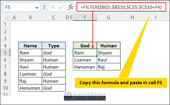
  =FILTER($B$5:$B$10,$C$5:$C$10=F4)
  Do the following to your desired list.
  >> Write “God” in cell F4 and “Human” in cell G4.
  >> Copy the above formula and paste it into cell F5 (it will list God Names)
  >> Similarly generate the Human Names. Just use G4 instead of F4 in the given formula.
  
  Can you visualize what to do? Please let us know if this helps.
  Regards
  -ExcelDemy Team
  - Reply
    Rene Feb 2, 2024 at 10:59 PM
    
    When I copy and paste your formula, it responds great for the first 8 rows. When I expand to include cells B5:B144 and C5:C144 it returns #N/A. Can you please help?
    
    Thank You
    - Lutfor Rahman Shimanto Feb 4, 2024 at 3:53 PM
      
      Hello RENE
      
      Thanks for reaching out and sharing your problem. You have observed that the formula works for the first eight rows. When you expand to include cells B5:B144 and C5:C144, it returns #N/A. However, our machine works perfectly fine, even though we work with an extensive range. The FILTER function is only available in Excel for Microsoft 365 and Excel 2021. Assuming you are using one of these versions.
      
      To resolve your problem, double-check the references in the formula to ensure they correspond to the correct columns and cells. Confirm that the formula is entered correctly without any typos or syntax errors. Good luck.
      
      Regards
      Lutfor Rahman Shimanto
      ExcelDemy
Darrell Mar 24, 2023 at 4:07 AM

I’m not sure if this is the best option for my need. I am being told I will be given a project next week where a list of materials will result from multiple selections that are setup in pick lists. I can setup the pick lists but will need some advice on how to get resulting list, based on what selections were made. I would love some advice.
- Reply
  Rafiul Hasan Mar 27, 2023 at 12:17 PM
  
  Hi DARRELL,
  Congratulations on your new project. Be confident, you can make it. Based on your selections, you may use any of the following to get resulting list:
  1. IF function: You can use the “IF” function to create a formula that checks if certain criteria are met and return the appropriate value. For example, if you have a pick list for materials and another for color, you can use an “IF” function to generate a list of materials that match the selected color.
  2. VLOOKUP function: The “VLOOKUP” function can be used to search for a value in a table and return a corresponding value. You can set up a table with all the possible combinations of selections and use “VLOOKUP” to generate the resulting list based on the selections made.
  3. FILTER function: The “FILTER” function can be used to filter a list based on certain criteria. You can set up a table with all the materials and their attributes (such as color, size, etc.) and use “FILTER” to generate a list of materials that match the selected attributes.
  4. PivotTable: Pivot tables can be used to analyze and summarize data in a table. you can set up a table with all the selections made and your corresponding materials and use a pivot table to generate a list of materials based on the selections made.
  
  These are just a few options you can consider. You will need to choose the one that works best for your specific situation. Don’t hesitate to contact with us if you face any problem. Best of luck.
  
  Regards
  Rafiul Hasan
  Team ExcelDemy
RENAE HINES Oct 12, 2023 at 9:30 PM

Hello,

My questions is I want to create a checklist that if I choose one of the options it brings up the tasks for that option. For example, my choices would be green or blue. If I choose blue, it has it’s own tasks that differ than green. How would I go about doing that?
- Reply
  Afrina Nafisa Oct 15, 2023 at 3:12 PM
  Hello RENAE HINES,
  
  Hope you are doing well. Thank you for your query. You can create a dynamic checklist using Excel’s built-in feature such as Data Validation.
  - Initially, select cell E5 and go to Data >> Data Tools >> Data Validation to get the particular color.
  - Then, Data Validation dialog box will pop up. Select List from the drop-down menu of Validation criteria and Source as E14:E15.
  - Lastly, Click OK to complete the Data validation process.
  - Here, the process of selecting color is dynamic as below.
  - Finally, enter the below formula in cell E6 to complete the dynamic checklist of getting task colorwise.
  =FILTER($C$5:$C$16,EXACT($B$5:$B$16,E5))
Kay D Aug 15, 2024 at 2:33 AM

When I use method 1, it will work if I have a smaller number of cells, but I am attempting to index a list of 248 recipes by protein. When I go for the whole list, the index is pulling the recipe from above the date i’m looking for. Do you happen to know why?
- Reply
  Shamima Sultana Aug 15, 2024 at 1:33 PM
  
  Hello Kay D,
  
  The issue with using 248 rows in your INDEX and SMALL formula is not the problem, as Excel can handle thousands of rows in such functions. It sounds like the issue may be related to how the INDEX and SMALL functions are handling the range of cells. If the formula is getting values from the wrong row, there could be a mismatch between the row numbers used in the SMALL function and the actual row numbers in your data.
  
  Make sure that the ranges in your formula are correctly aligned with your dataset. Double-check that the criteria and ranges match, and ensure there are no offset errors.
  
  Adjust the “-4” ensure that the offset corresponds to the starting row of your range. Try modifying the offset if necessary, depending on your data structure.
  Check Criteria Range: Ensure the $C$5:$C$12 range is aligned with your criteria column.
  
  You can share your formula if you want. We can help to troubleshoot it further!
  
  Regards
  ExcelDemy
tallnsknny Jan 12, 2025 at 8:57 AM

I have Excel 2016 so I’m using Method 1 to create my list. One of the unique things I am doing is referencing a list from a different tab of the same file. The formula works fine in the first cell, but when I copy it down it comes up with blanks (I assume the error message). I assume you might want to see my spreadsheet? If so, do I mail it somewhere?
- Reply
  Shamima Sultana Jan 12, 2025 at 10:40 AM
  
  Hello Tallnsknny,
  
  Thank you for your comment! Referencing a list from a different tab should work fine with Method 1. If the formula returns blanks when copied down, it may be due to relative references not adjusting correctly. Try using absolute references $Sheet1!$A$1:$A$10 in your formula where necessary.
  
  If you’d like us to review your spreadsheet, you can share it by ExcelDemy Forum. Let us know if this helps!
  
  Regards
  ExcelDemy