Method 1 – Creating a Drop-Down List from Range
The following sample dataset will be used for illustration.
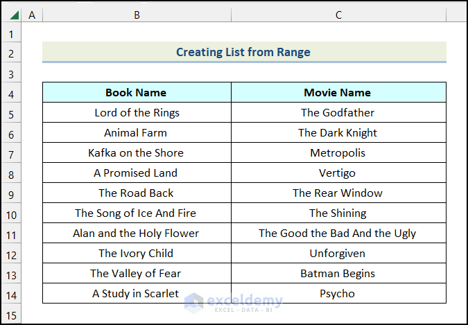
1.1 Independent Drop-Down List
Steps:
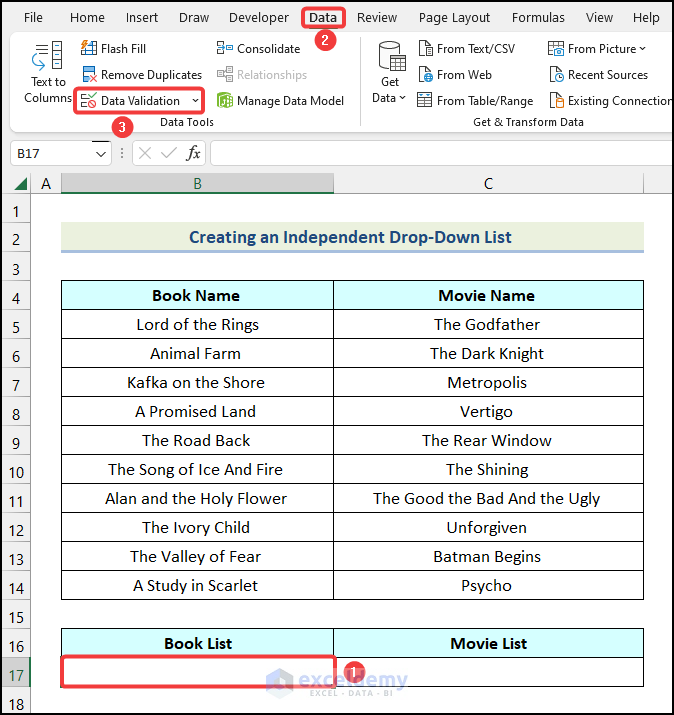
- Select the cell where you want to create the drop-down list. We have selected cell B17.
- Go to the Data tab from ribbon.
- Choose the Data Validation option from the Data Tools group.
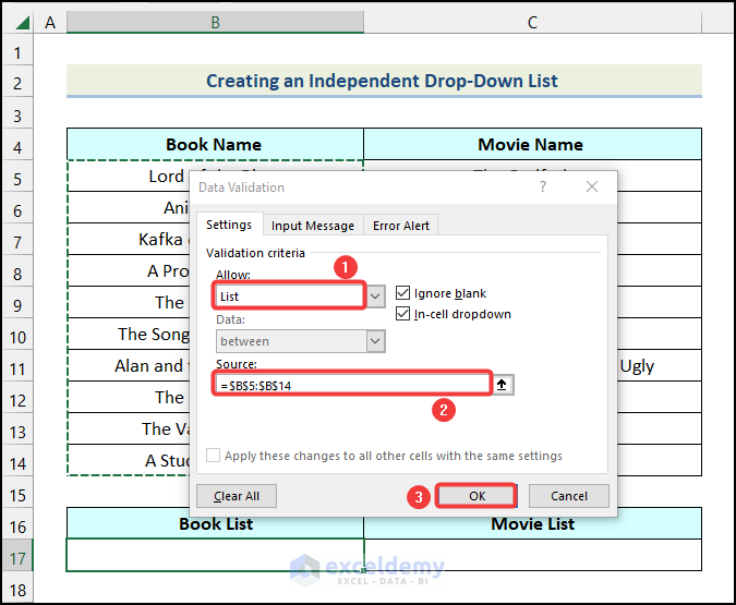
- In the Data Validation dialog box, choose the List option in the Allow field.
- In the Source field, select the range of cells B5:B14.
- Click OK.
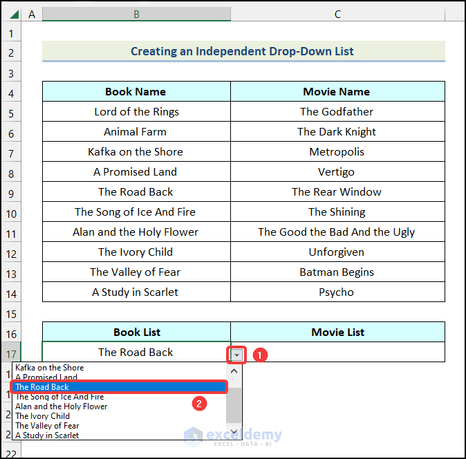
A drop-down icon will appear beside cell B17 as shown in the following image.
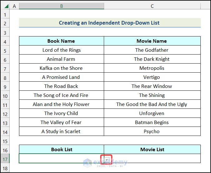
- Click on the drop-down icon.
- Select any name of the book from the drop-down. We have selected the book The Road Back.
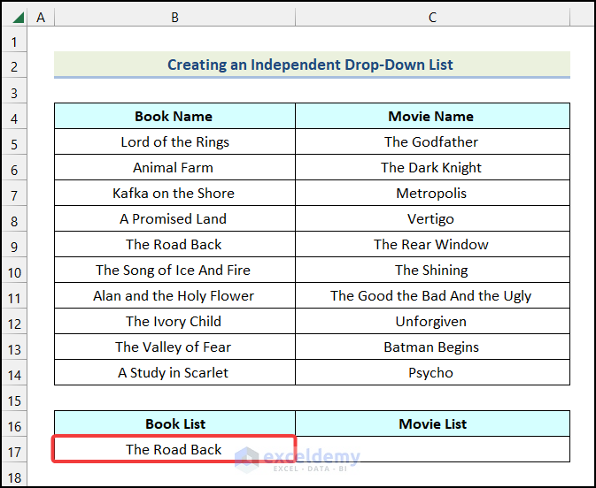
You will get the following output in your worksheet.
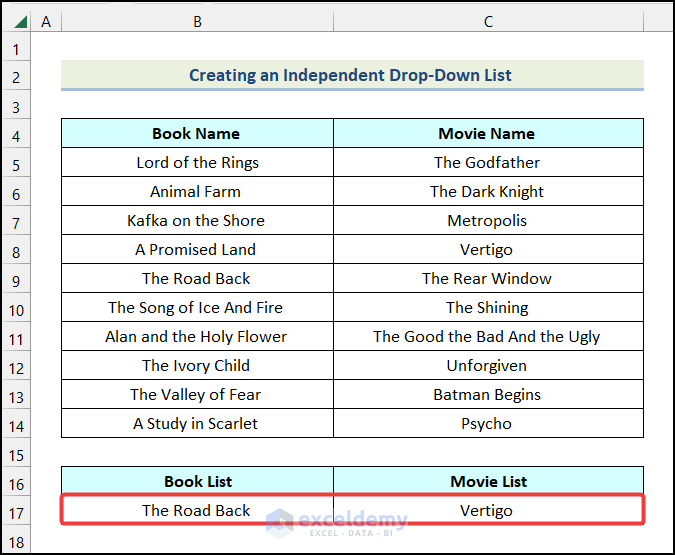
- Follow the same procedure for creating a drop-down list for the Movie Names and you will get the following output on your worksheet.
1.2 Dynamic Drop-Down List
A dynamic drop-down list will auto-update your data. When we delete some of the data from the dataset, the drop-down list will automatically update according to the change in the dataset.
Steps:
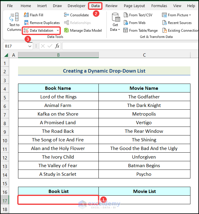
- Select the cell where you want to create the drop-down list. We have selected cell B17.
- Go to the Data tab from Ribbon.
- Choose the Data Validation option from the Data Tools group.
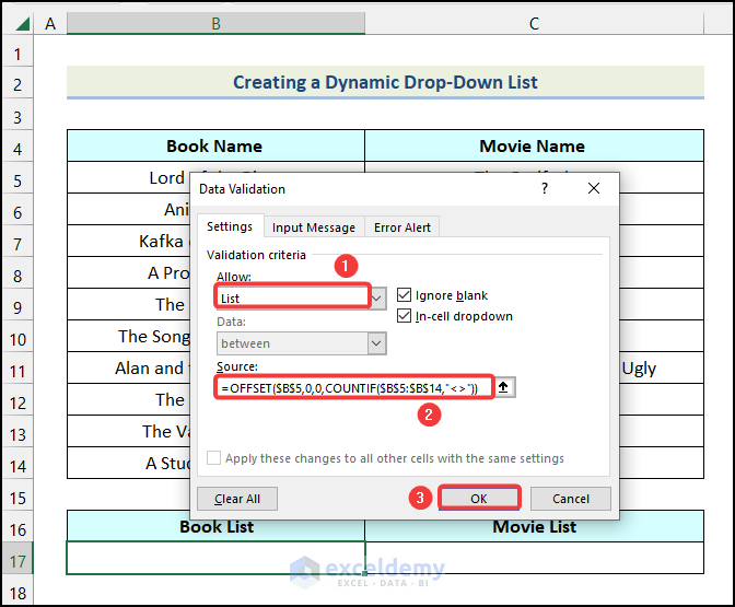
- In the Data Validation dialog box, choose the List option in the Allow field.
- In the Source field, enter the following formula.
=OFFSET($B$5,0,0,COUNTIF($B$5:$B$14,"<>"))Cell $B$5 indicates the first cell of the Book Name column and the range of cells $B$5:$B$14 denotes all of the cells of the Book Name column.
- Click OK.
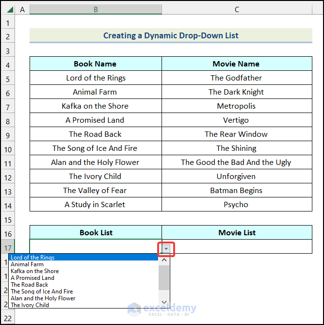
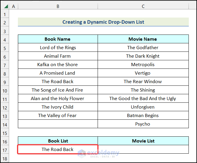
Consequently, a drop-down icon will appear beside cell B17, as shown in the following image.
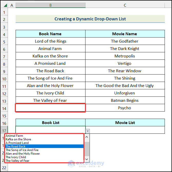
- Delete a cell from the Book Name We have deleted the last cell of the Book Name column which is A Study in Scarlet.
You will see that A Study in Scarlet is no longer available in the drop-down list.
- Click on the drop-down icon.
- Select any name of the book from the drop-down. We have selected the book The Road Back.
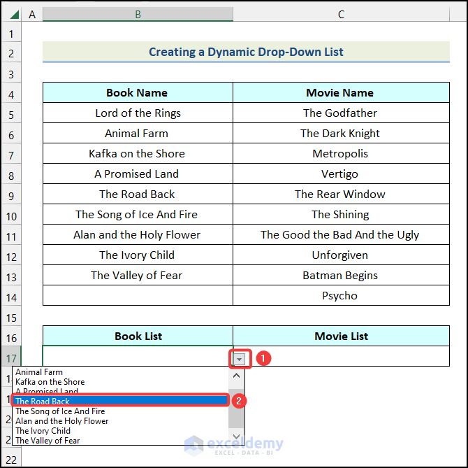
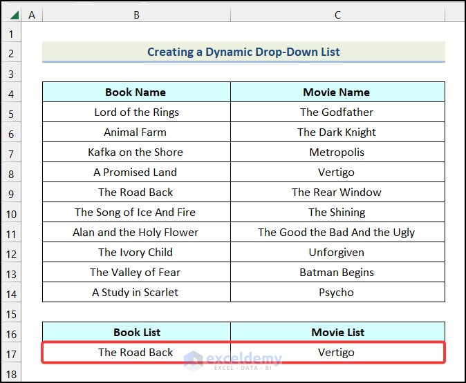
You will get the following output in your worksheet.
- Follow the same procedure for creating a drop-down list for the Movie Names and you will get the following output on your worksheet.
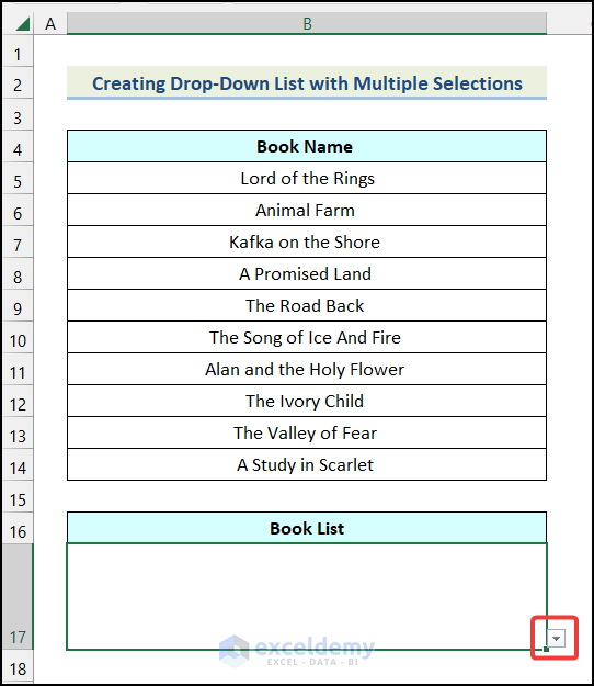
1.3 Drop-Down List with Multiple Selections
Steps:
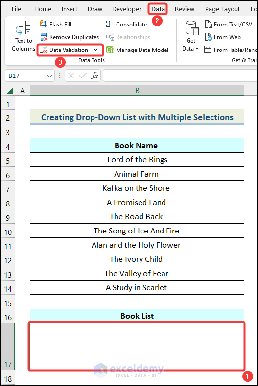
- Select the cell where you want to create the drop-down list. We have selected cell B17.
- Go to the Data tab from ribbon.
- Choose the Data Validation option from the Data Tools group.
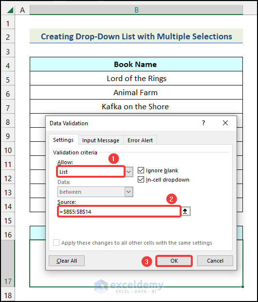
- In the Data Validation dialog box, choose the List option in the Allow field.
- In the Source field, select the range of cells B5:B14.
- Click OK.
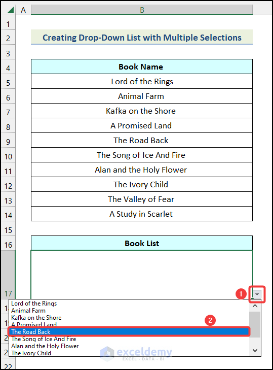
A drop-down icon will appear beside cell B17 as shown in the following image.
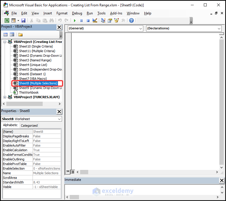
- Use the keyboard shortcut ALT + F11 to open the Microsoft Visual Basic window.
- In the Microsoft Visual Basic window, find the name of the worksheet that you are currently using. In this case, it is Multiple Sections.
- Double-click on the name of the worksheet.
- Enter the following code.
Option Explicit
Private Sub Worksheet_Change(ByVal target_value As Range)
Dim prev_value As String
Dim current_value As String
Application.EnableEvents = True
On Error GoTo Exitsub
If Not Intersect(target_value, Range("B17")) Is Nothing Then
  If target_value.SpecialCells(xlCellTypeAllValidation) Is Nothing Then
    GoTo Exitsub
  Else: If target_value.Value = "" Then GoTo Exitsub Else
    Application.EnableEvents = False
    current_value = target_value.Value
    Application.Undo
    prev_value = target_value.Value
      If prev_value = "" Then
        target_value.Value = current_value
      Else
        If InStr(1, prev_value, current_value) = 0 Then
            target_value.Value = prev_value & vbNewLine & current_value
      Else:
        target_value.Value = prev_value
      End If
    End If
  End If
End If
Application.EnableEvents = True
Exitsub:
Application.EnableEvents = True
End Sub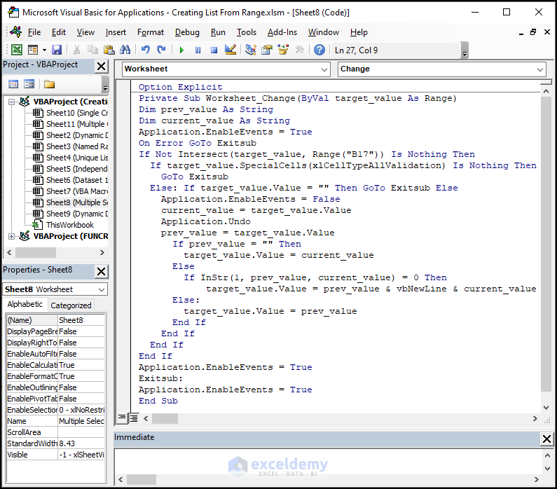
Code Breakdown
- We have initiated a sub-routine named Worksheet_Change.
- Inside the function argument, we have specified the target_value as Range.
- We have declared two variables named prev_value and current_value as String.
- We have used an IF statement to specify the output cell.
- We have used another IF statement to make sure that this VBA code only works for those cells which have data validation enabled in them.
- We have assigned the value of the target_value variable to the current_value variable.
- We have used another IF statement to check if the value of the prev_value argument is “” or not.
- If this condition is satisfied, then the value of the current_value variable will be assigned to the target_value variable.
- We have used the VBA InStr function in another IF statement to check whether the output of the InStr function in 0 or not.
- If the output is 0, then both the prev_value and current_value will be assigned to the target_value variable with a line break.
- Otherwise, prev_value will be assigned to the target_value variable.
- We have closed the IF statements.
- We have ended the sub-routine.
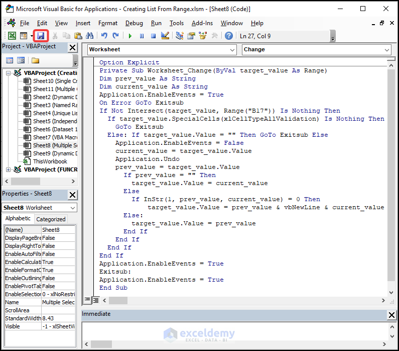
- Click on the Save
- Click on the drop-down icon beside cell B17.
- Choose a Book Name form the drop-down list. In this case, we selected the book named The Road Back.
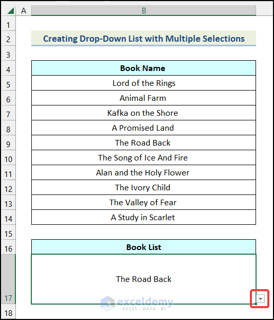
The name of the book will appear in cell B17 as shown in the following image.
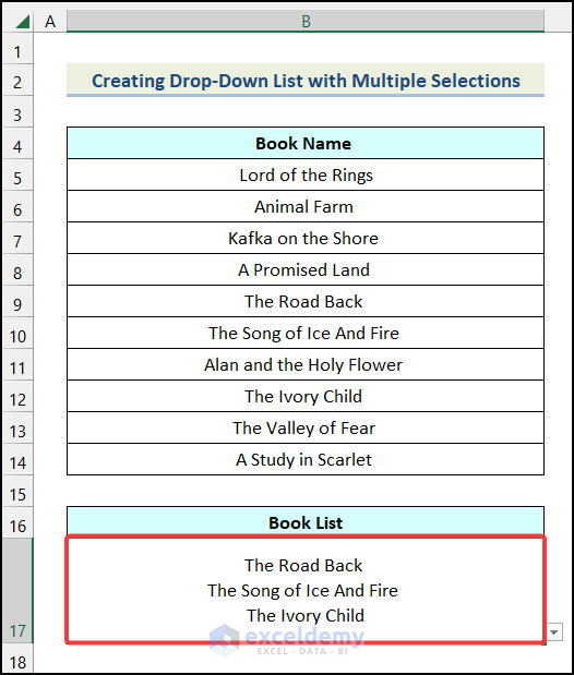
- Add more Book Names to the list.
You will have the following outputs on your worksheet as shown in the following image.
Read More: How to Make a List within a Cell in Excel
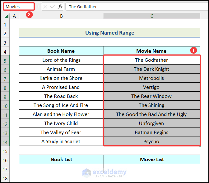
Method 2 – Using Named Range
Steps:
- Select the range of cells that you want to include in the drop-down list. We have selected cells B5:B14.
- Define a suitable name inside the marked box as shown in the following image. We have used the name Books to name our range.
Note: While naming ranges, spaces are not allowed between multiple words.
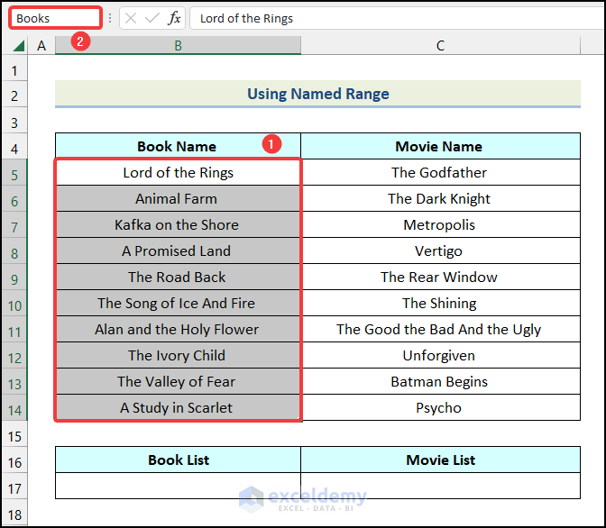
- Name the cell range C5:C14. We have used the name Movies to name this range.
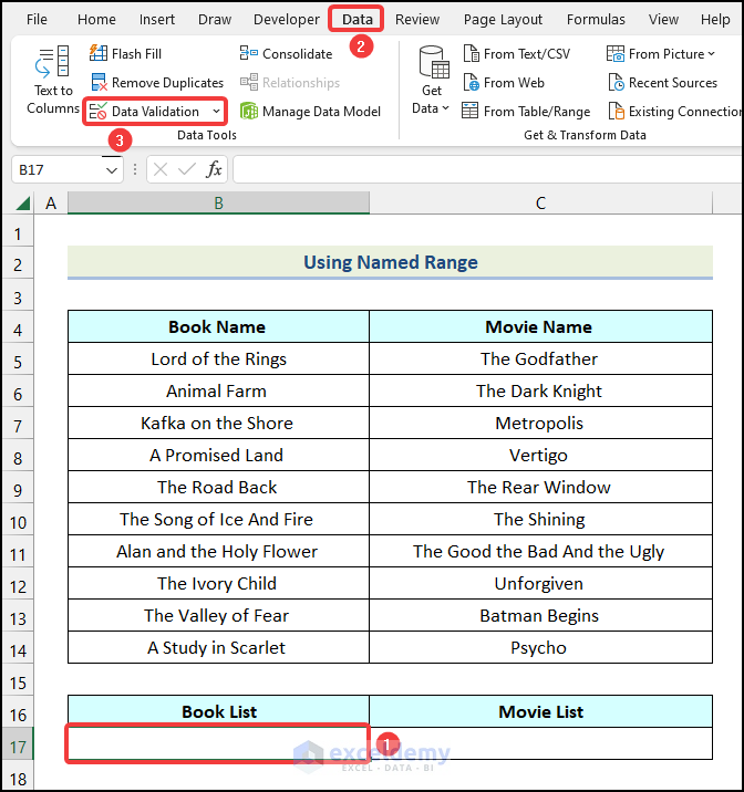
- Select the cell where you want to create the drop-down list. We have selected cell B17.
- Go to the Data tab from Ribbon.
- Choose the Data Validation option from the Data Tools group.
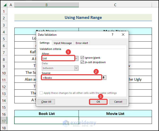
- In the Data Validation dialog box, choose the List option in the Allow field.
- In the Source field, select the range of cells B5:B14.
- Click OK.
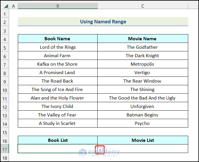
A drop-down icon will be available beside cell B17 as shown in the following image.
- Click on the drop-down icon.
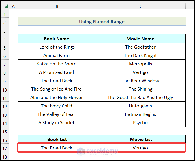
- Select any name of the book from the drop-down. We have selected the book, The Road Back.
- Follow the same steps to create a list from the range of cells C5:C14 and you will have the following output.
Method 3 – Creating List from Range Based on Criteria
3.1 Creating List Based on a Single Criterion
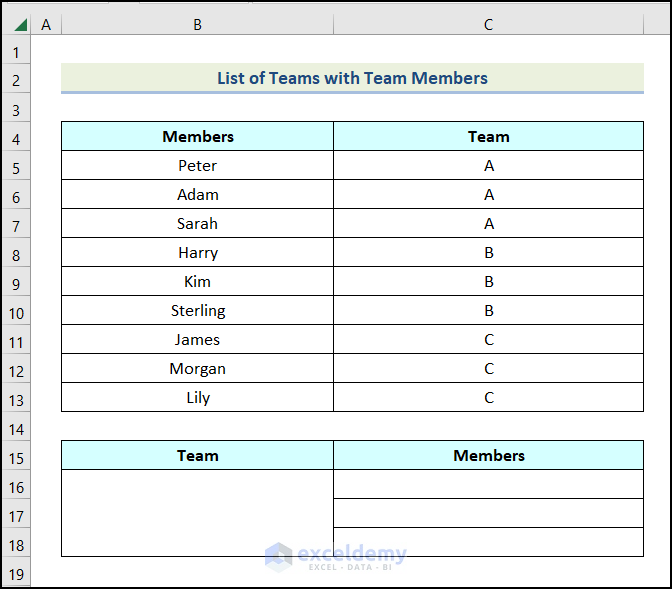
We have the List of Teams with Team Members as our sample dataset. We will create a list of Team Members based on the selected Team.
Steps:
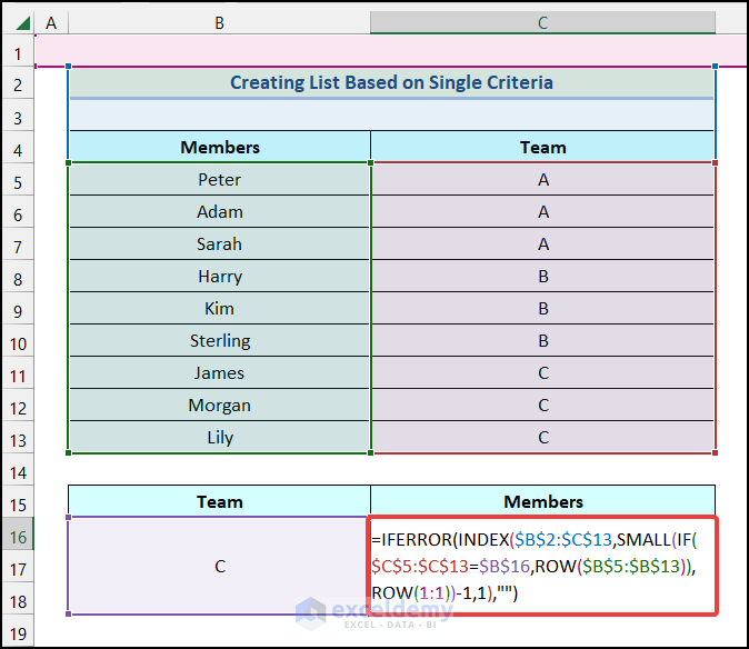
- Enter the following formula in cell C16.
=IFERROR(INDEX($B$2:$C$13,SMALL(IF($C$5:$C$13=$B$16,ROW($B$5:$B$13)),ROW(1:1))-1,1),"")The range of cells $B$2:$C$13 indicates the entire dataset, range $C$5:$C$13 refers to the cells of the column named “Team” cell $B$16 represents the selected “Team”, and range $B$5:$B$13 refers to the cells of the column named “Members”.
Formula Breakdown
- In the first ROW function ROW($B$5:$B$13),
- $B$5:$B$13 → It is the [reference] argument.
- Output → {5;6;7;8;9;10;11;12;13}.
- In the IF function IF($C$5:$C$13=$B$16,ROW($B$5:$B$13)),
- $C$5:$C$13=$B$16 → It denotes the logical_test argument.
- ROW($B$5:$B$13) → This represents the [value_if_true] argument.
- Output → {FALSE;FALSE;FALSE;FALSE;FALSE;FALSE;11;12;13}.
- The SMALL function becomes → SMALL({FALSE;FALSE;FALSE;FALSE;FALSE;FALSE;11;12;13},ROW(1:1))
- Here, {FALSE;FALSE;FALSE;FALSE;FALSE;FALSE;11;12;13} → This is the array argument.
- ROW(1:1)) → This indicates the k argument.
- Output → {11}.
- The INDEX function, INDEX($B$2:$C$13,SMALL(IF($C$5:$C$13=$B$16,ROW($B$5:$B$13)),ROW(1:1))-1,1) becomes → INDEX($B$2:$C$13,{11}-1,1).
- Here, $B$2:$C$13 → It is the array argument.
- {11}-1 → This denotes the row_num argument.
- 1 → It is the column_num argument.
- Output → “James”.
- The IFERROR function becomes =IFERROR(“James”,””).
- Here, “James” → It indicates the value argument.
- “” → This refers to the [value_if_error] argument.
- Output → James.
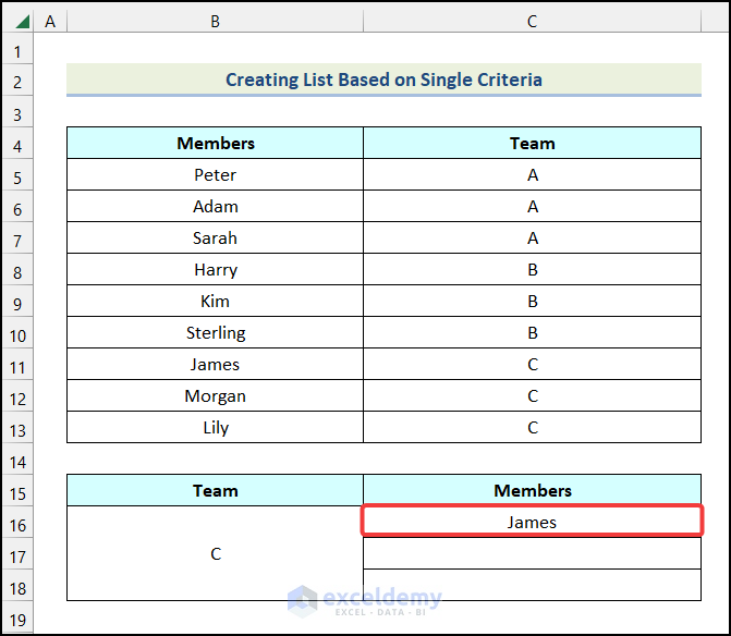
- Press ENTER.
You will get the following output in cell C16.
- Use the AutoFill option to get the remaining outputs as shown in the following image.
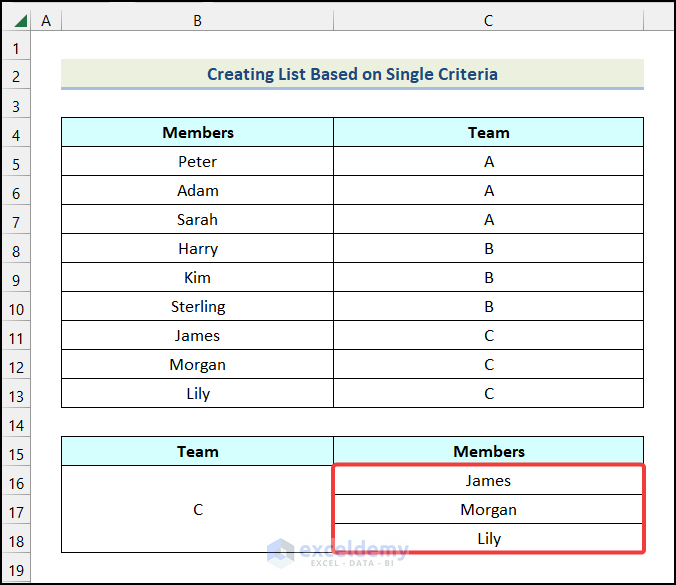
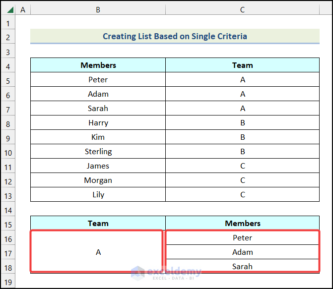
Change the name of the Team from C to A and the outputs will be changed automatically.
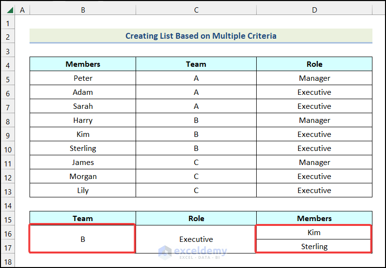
3.2 Creating List Based on Multiple Criteria
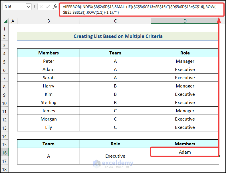
In the following sample dataset, we have the names of Team Members with Team names along with their Roles. We will create a list based on the selected Team name and Role.
Steps:
- Add the following formula in cell D16.
=IFERROR(INDEX($B$2:$D$13,SMALL(IF(($C$5:$C$13=$B$16)*($D$5:$D$13=$C$16),ROW($B$5:$B$13)),ROW(1:1))-1,1),"")- Press ENTER.
You will have the name of a team member from Team A and the Role of Executive.
- Use the Fill Handle tool for the remaining cells.
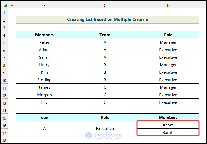
You can change the criteria according to your need and the output will be adjusted automatically.
Read More: How to Generate List Based on Criteria in Excel
Method 4 – Generating List Using VBA Macro Feature
Steps:
- Press ALT + F11 to open the Microsoft Visual Basic window.
- In the Microsoft Visual Basic window, find the name of the worksheet that you are currently using. In this case, it is VBA Macro.
- Double-click on the name of the worksheet.
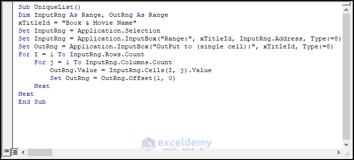
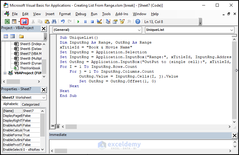
- Add the following code.
Sub UniqueList()
Dim InputRng As Range, OutRng As Range
xTitleId = "Book & Movie Name"
Set InputRng = Application.Selection
Set InputRng = Application.InputBox("Range:", xTitleId, InputRng.Address, Type:=8)
Set OutRng = Application.InputBox("OutPut to (single cell):", xTitleId, Type:=8)
For I = 1 To InputRng.Rows.Count
    For j = 1 To InputRng.Columns.Count
        OutRng.Value = InputRng.Cells(I, j).Value
        Set OutRng = OutRng.Offset(1, 0)
    Next
Next
End Sub
Code Breakdown
- We have created a sub-routine named UniqueList.
- We have introduced two variables named InputRng and OutRng as Range.
- We have specified the title for the message box that will appear when running the macro.
- We have used Set statements to define the InputRng and the OutRng.
- We have initiated a For Next loop from 1 to the number of rows in the input range.
- We have started another For Next loop from 1 to the number of columns in the input range.
- We have assigned the cells of the InputRng to the OutRng.
- We have used the OFFSET function with a Set statement to define the OutRng variable.
- We have ended the For Next
- We have ended the sub-routine.
- After entering the code, click on the Save icon as shown in the following image.
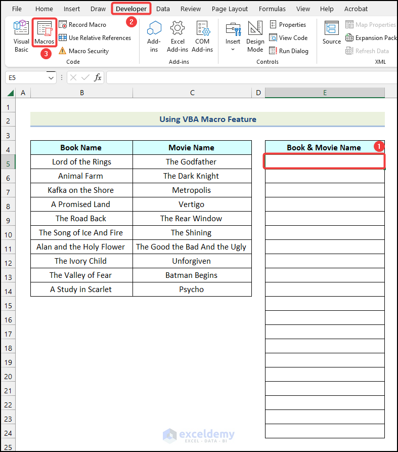
- Select the cell where you want to create the list. We have selected cell E5.
- Go to the Developer tab from Ribbon.
- Choose the Macros option from the Code group.
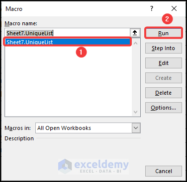
- In the Macro dialog box, click on UniqueList option.
- Click on Run.
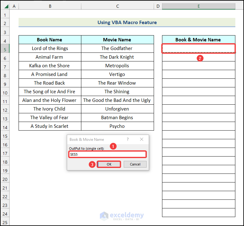
A dialog box, Book & Movie Name will pop up.
- Select the entire dataset and click OK.
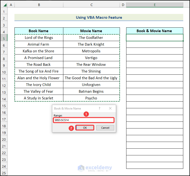
- Select the destination cell of the outputs. We have selected cell E5.
- Click OK.
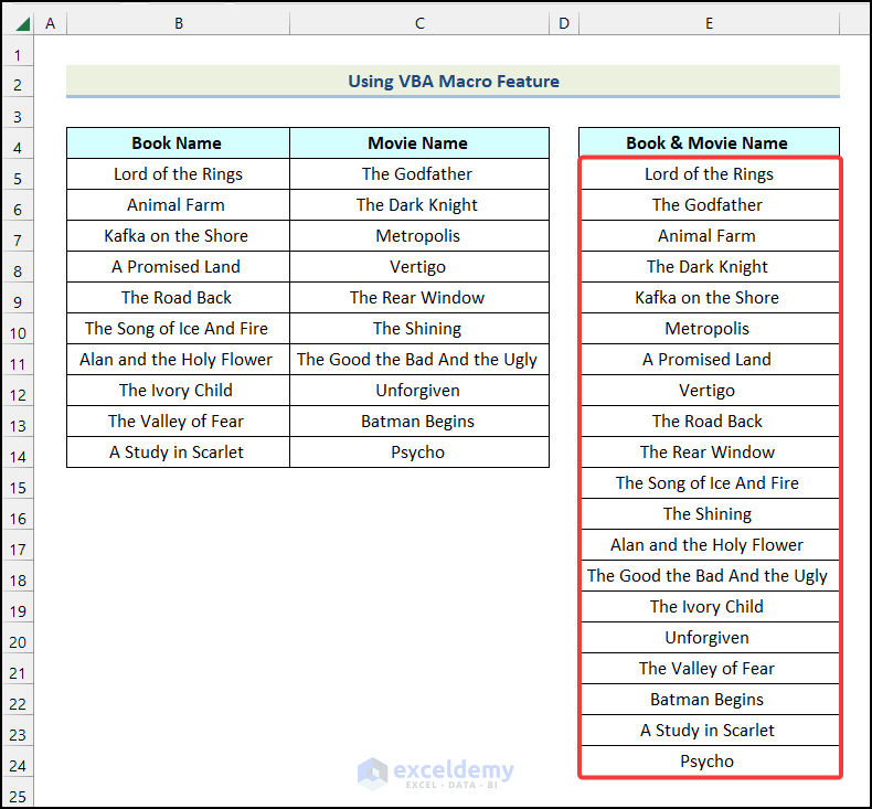
The list of Book Name and Movie Name will appear in the Book & Movie Name column as shown in the following image.
How to Create a Unique List from Range in Excel
We can create a unique list based on criteria from the range in Excel. We will use the UNIQUE function to create a unique list.
Note: The UNIQUE function is available in Excel 2021 and in Excel 365.
Steps:
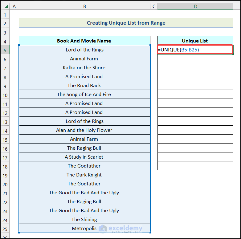
- Add the formula given below in cell D5.
=UNIQUE(B5:B25)The range of cells B5:B25 indicates the cells of columns Book and Movie Name.
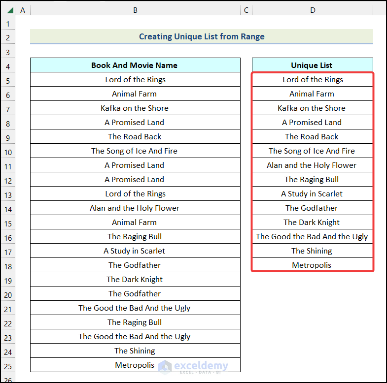
- Press ENTER.
You will get a list of unique cells from the range B5:B25 as shown in the following image.
Read More: How to Make a Numbered List in Excel
Download Practice Workbook
Similar Articles for You to Explore
- How to Make a To Do List in Excel
- How to Create a Contact List in Excel
- How to Make a Comma Separated List in Excel
- How to Make a Price List in Excel
<< Go Back to Make List in Excel | Excel Drop-Down List | Data Validation in Excel | Learn Excel
Get FREE Advanced Excel Exercises with Solutions!
