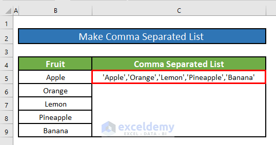
We have an Excel file that contains information about various types of fruits. These fruits are listed in the column titled Fruit in that Excel worksheet. We will make this column of fruits into a comma-separated list. Here’s an overview of the dataset.
Method 1 – Use the CONCATENATE Function to Make a Comma-Separated List in Excel
Steps:
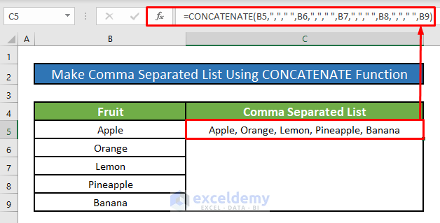
- Use the following formula in cell C5.
=CONCATENATE(B5,","," ",B6,","," ",B7,","," ",B8,","," ",B9)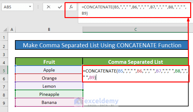
- Press Enter.
Read More: How to Make a To Do List in Excel
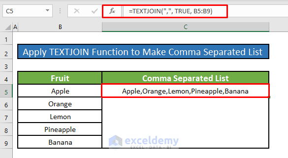
Method 2 – Apply the TEXTJOIN Function to Make a Comma-Separated List in Excel
Steps:
- Use the following formula in cell C5.
=TEXTJOIN(“,”, B5:B9)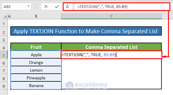
- Press Enter.
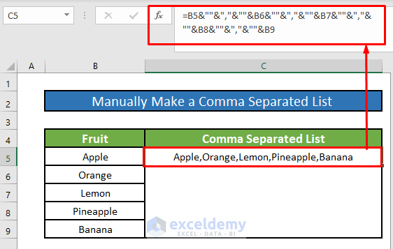
Method 3 – Use a Custom Formula to Make a Comma Separated List in Excel
Steps:
- Select cell C5 and insert the following formula in the formula bar:
=B5&""&","&""&B6&""&","&""&B7&""&","&""&B8&""&","&""&B9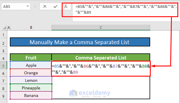
- Press Enter.
Read More: How to Make a List within a Cell in Excel
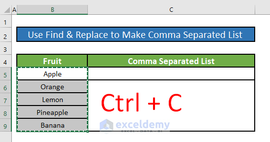
Method 4 – Use the Find & Replace Command to Make a Comma Separated List in Excel
Steps:
- Select all the cells in the Fruit column except the column header.
- Press Ctrl + C on your keyboard simultaneously to copy these cells.
- Paste the copied cells into a blank Microsoft Word document with Ctrl + V.
- You’ll get a dropdown option named Paste Options (Ctrl) on the bottom-right corner of the pasted cells.
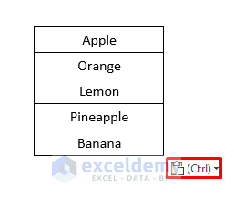
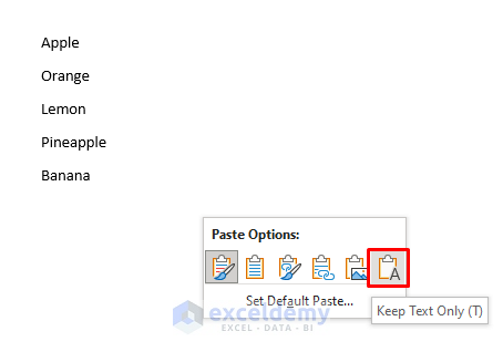
- Click on the Paste Options and select Keep Text Only.
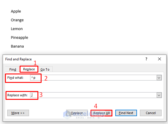
- Press Ctrl + H to open the Find and Replace box.
- Insert “^p” in the Find what input box.
- Enter “,” in the Replace with input box.
- Click on the Replace All button.
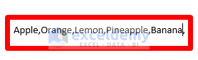
- All cell values in the Fruit column are converted to a comma-separated list in Microsoft Word.

- Here’s the resulting list.
Read More: How to Generate List Based on Criteria in Excel
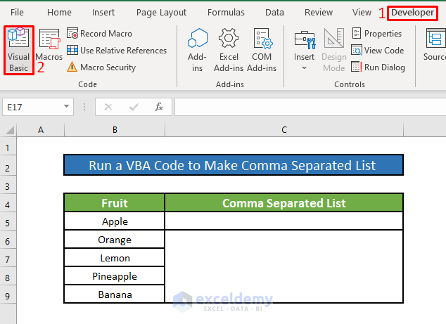
Method 5 – Run VBA Code to Make a Comma Separated List in Excel
Steps:
- Go to the Developer tab and select Visual Basic.
- A window named Microsoft Visual Basic for Applications will appear.
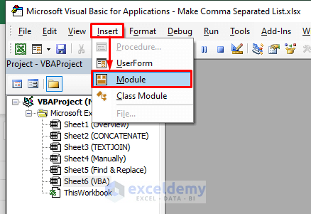
- Insert a module by going to Insert and selecting Module.
- In the module, insert the following VBA code.
Function ColumntoList(ColRange As Range)
            Dim ListOutput
            Dim cell As Variant
            For Each cell In ColRange
            If Not IsEmpty(cell.Value) Then
            ListOutput = ListOutput & "'" & cell.Value & "',"
            End If
            Next
            ColumntoList = Left(ListOutput, Len(ListOutput) - 1)
End Function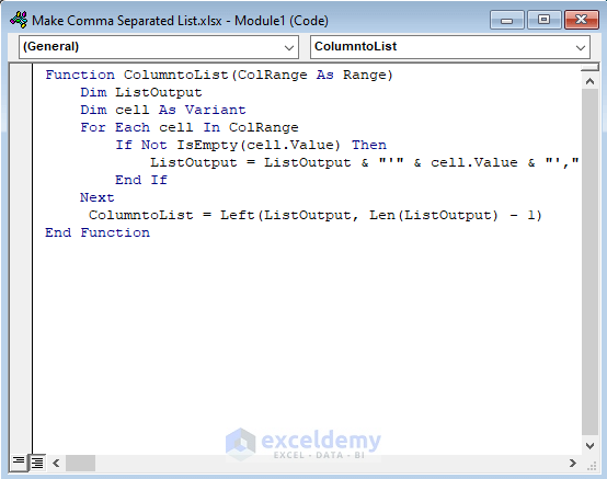
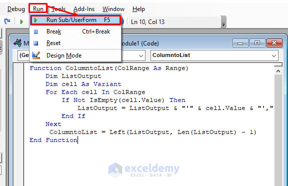
- Run the VBA by pressing the Play button or F5.
- Go back to the worksheet and use the following formula in cell C5.
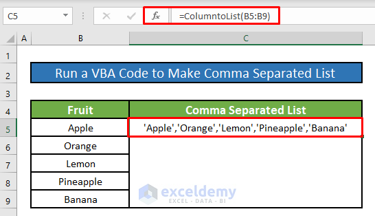
=ColumntoList(B5:B9)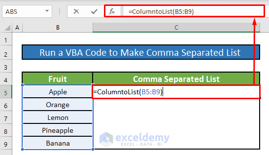
- Press Enter and you will get your desired output in cell C5.
Read More: How to Create List from Range in Excel
Things to Remember
If the Developer tab is not visible in your ribbon, you can make it visible. To do that, go to File → Option → Customize Ribbon.
Download the Practice Workbook
Related Articles
- How to Make a Numbered List in Excel
- Create a Unique List in Excel Based on Criteria
- How to Make a Price List in Excel
- How to Create a Contact List in Excel
<< Go Back to Make List in Excel | Excel Drop-Down List | Data Validation in Excel | Learn Excel
Get FREE Advanced Excel Exercises with Solutions!

Thank you for this guide, it worked perfectly for me. The instructions and step by step screenshots are clear and easy to understand. I learned a lot from this guide.
Hello, Eric!
Thanks for your appreciation. To get more helpful content stay in touch with ExcelDemy.
Regards
ExcelDemy
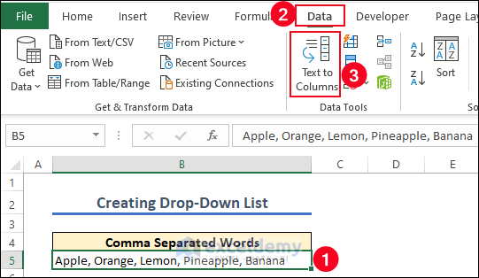
What I’m searching for is the other way around. So I have one cell with comma separated words, and I would like excel to take all those words and create a dropdown menu (list) from that, instead of creating a dropdown list from a colomn.
Hello TOM DE JONGH!
Thanks for your query.
You have one cell with comma-separated words, and create a dropdown menu (list) from that, instead of creating a dropdown list from a column.
We will convert those comma-separated words into columns using the Text to Columns feature. Hence, transpose these words using the TRANSPOSE function. After that, we will create a drop-down list using the Data Validation feature.
Let’s follow the instructions below to learn!
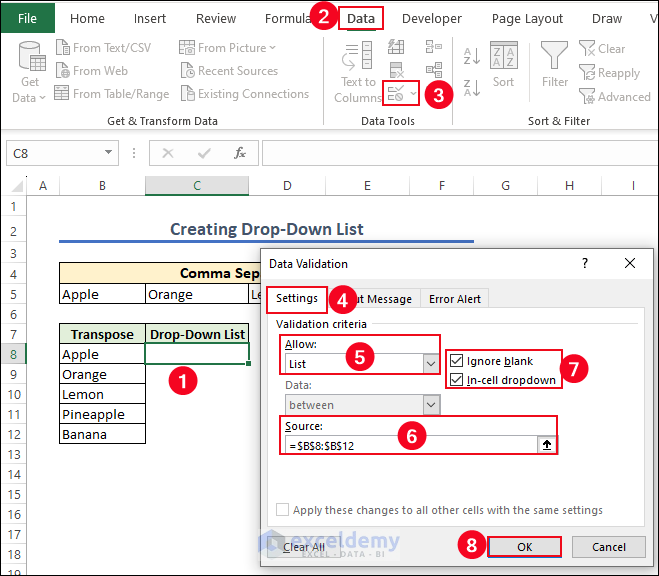
To split the comma-separated words, go to,
Data >> Data Tools >> Text to Columns
We will use the comma as a delimiter.
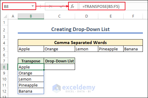
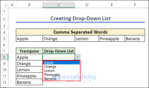
Hence, you will be able to split the comma-separated words and then in cell B8 apply the TRANSPOSE function to transpose row to column.
=TRANSPOSE(B5:F5)Now, we’ll select cell C8 to create the drop-down list using the Data Validation feature.
Finally, you will be able to create a drop-down menu from a comma-separated words cell.
Please download the Excel file to solve your problem and practice with it.
Creating Drop-Down List.xlsx
Now I think you can solve your problem. If you cannot solve your problem, you can contact with us via this mail [email protected]
Regards
Md. Abdur Rahim Rasel
Exceldemy Team