Method 1 – The Data Analysis Tool as a Random Number Generator in Excel
Steps:
- Go to the tab Data -> Data Analysis.
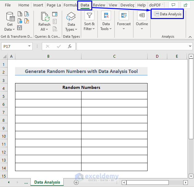
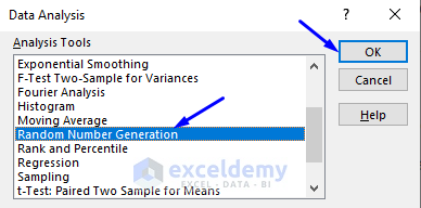
- From the Data Analysis pop-up box, select Random Number Generation.
- Click OK.
- Another Random Number Generation pop-up box will appear.
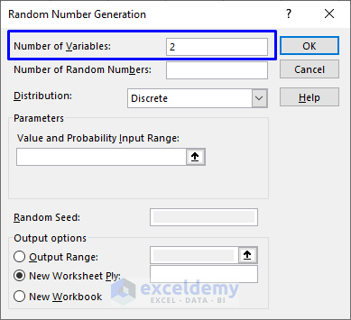
- In the Number of Variables section, write the number of columns in which you want to generate random numbers to generate random numbers in 2 columns, Column B and Column C. We wrote 2 in there.
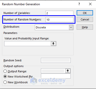
- The Number of Random Numbers section, write the number of random numbers you want to generate. For example, we wanted to generate 10 random numbers, so we wrote 10 in that box.
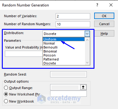
- There are 7 types of Distribution in random number generation. The types are:
- Uniform: To generate numbers from a specified low value to a high value.
- Normal: To generate numbers based on a specified range of Mean and Standard Deviation.
- Bernoulli: To generate numbers that have the probability of success either 0 or 1.
- Binomial: To generate numbers that have the probability of success for a number of trials.
- Poisson: To generate numbers based on Lambda value, fraction equal to 1/Mean.
- Patterned: To generate numbers that have a lower and upper limit, in a certain step and a fixed number of repetition periods for both the values and the sequence.
- Discrete: To generate numbers that have a value and probability. The sum of the probability is generally 1. To display results, it usually uses two columns.
We selected Uniform distribution. Select any distribution type according to your requirements.
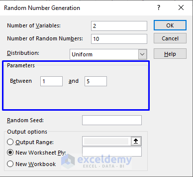
- The Parameters group will show up. Insert the low value and the high value in the appropriate boxes. We will generate random numbers from 1 to 5, so we wrote 1 and 5 in the Between section.
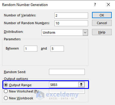
- Random Seed is usually used when we need to generate the same set of numbers. Random Seed keeps the data centered on the inserted values.
- Write the destination location in the Output Range to generate a random number in cell B5, so we selected that cell. Or you can write the cell reference address.
You can also place the newly generated numbers in a new worksheet or even a new workbook. Check the New Worksheet Ply or the New Workbook option from the pop-up box.
- Press OK.
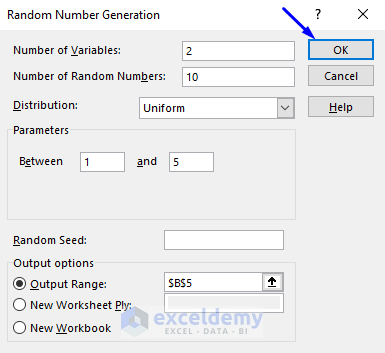
The following image has the outcome of all the steps executed.
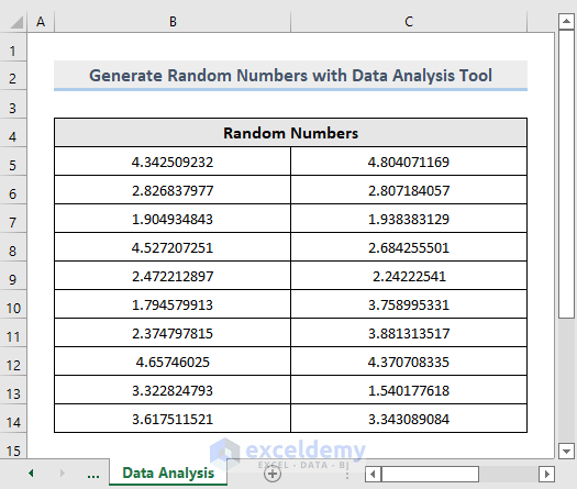
Random numbers from 1 to 5 in the specified location in our Excel dataset were successfully generated.
Method 2 – The RAND Function to Generate Random Numbers in Excel
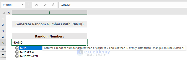
The RAND function returns a random number greater than or equal to 0 and less than 1. The numbers are evenly distributed, they change on every recalculation.
Steps:
- Pick a cell to store the number.
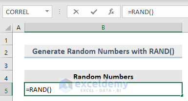
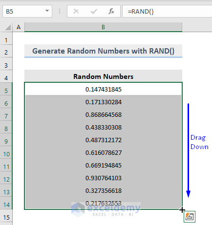
- In the cell, write the RAND function.
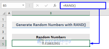
=RAND()- Press Enter.
- There will be a random number generated in that cell.
- Drag the cell down to produce as many random numbers as you want in the worksheet.
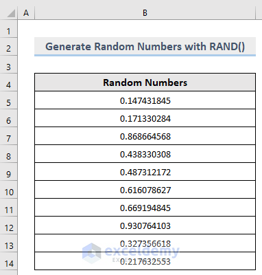
By following these steps, you can successfully generate random numbers from 0 to less than 1 with the RAND function in Excel.
Method 3 – The RANK.EQ Function as the Random Number Generator
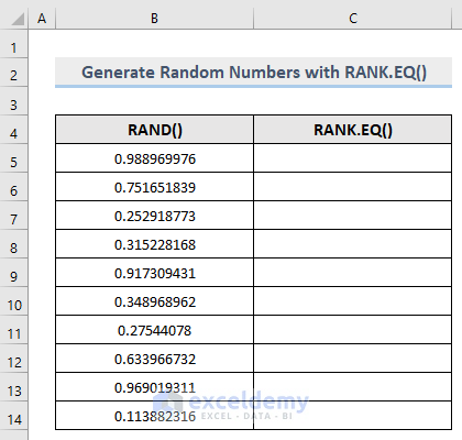
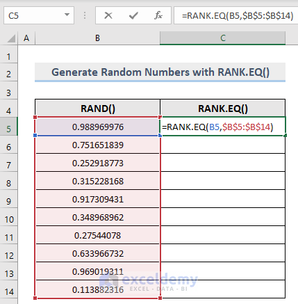
Utilize the RANK.EQ function to produce random numbers in Excel to produce random numbers with RANK.EQ, you have to have a source number list. We generated random numbers in the range B5:B14 with the RAND function, we will take that range as our source number list to generate random numbers in the range C5:C14 with the RANK.EQ function in Excel.
Steps:
- Pick a cell to store the first number of a list of numbers. We picked cell C5, the cell next to the first generated number from the RAND function. The RAND function generated the source range B4:B14.
- In that cell, write the RANK.EQ function. You will notice the parameters that you need to input inside the parentheses of the function.
- Pass a source number as the first parameter. The number is from cell B5.
- Pass the list of source numbers as the reference; it is in the range B5:B14.
- Order parameter is optional, if you want your data to be organized in Ascending or Descending format, then you should use this.
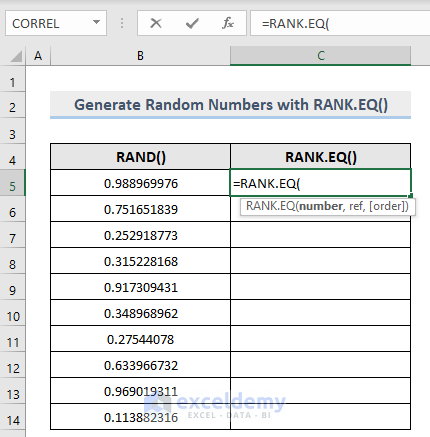
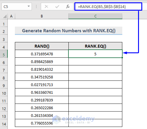
- The formula now becomes like this:
=RANK.EQ(B5,$B$5:$B$14)- Press Enter.
- A random number will be generated in that cell.
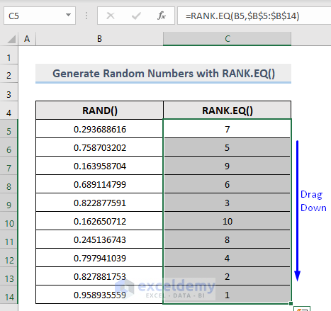
- Drag the cell down to produce the rank numbers based on the rank of the source number list in your worksheet.
Method 4 – RANDBETWEEN Function as Random Number Generator in Excel
The RANDBETWEEN function is another effective function to generate random numbers in Excel. It returns the random numbers between the specified numbers.
Steps:
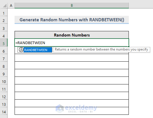
- Pick a cell to store the number. We picked cell B5.
- In that cell, write the RANDBETWEEN. You will notice the parameters that you need to input inside the function’s parentheses.
- bottom means the lower value. We define 5 as the low value for our dataset.
- top means the upper value. We declare 10 as the high value for our dataset.
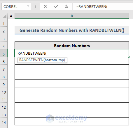
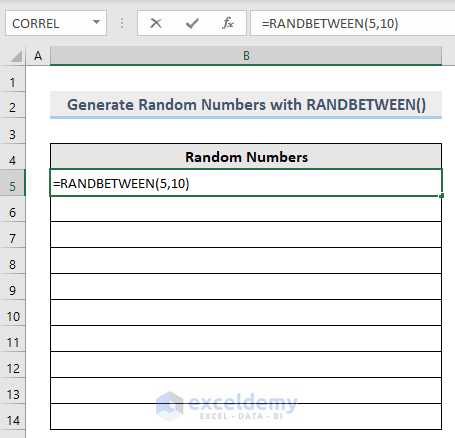
- The formula now becomes like this:
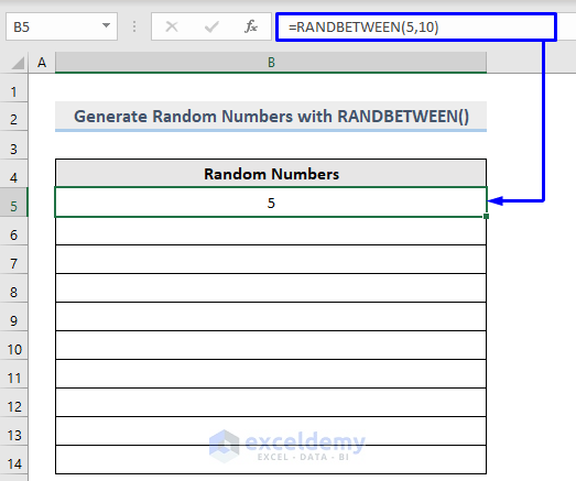
=RANDBETWEEN(5,10)- Press Enter.
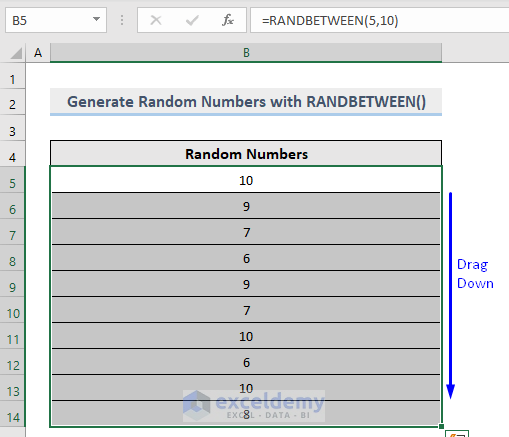
- A random number will be generated in that cell.
- Drag the cell down to produce random numbers between the numbers 5 and 10 in the worksheet.
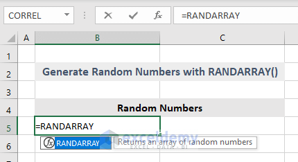
Method 5 – The RANDARRAY Function to Generate an Array of Random Numbers
The RANDARRAY function returns an array of random numbers in Excel.
Steps:
- Pick a cell to store the first number of an array of numbers.
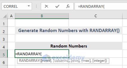
- In that cell, write the RANDARRAY, you will notice the parameters that you need to input inside the parentheses of the function.
- Pass rows – we want 5 rows to carry the numbers, so we pass 5 as the first parameter inside the parentheses of the function.
- Pass columns – we want 2 columns to carry the numbers, so we pass 2 as the second parameter.
- Pass min – the minimum value to generate numbers from 5, so 5 is the minimum value for our dataset.
- Pass max – the maximum value to generate numbers till 10, so 10 is the maximum value for our dataset.
-
- To return the result in the Decimal value, select FALSE, or if you want the result in the Integer value, then select The result in the Integer format, so we picked TRUE.
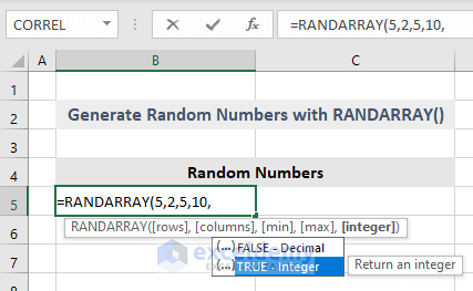
- The formula now becomes like this:
=RANDARRAY(5,2,5,10,TRUE)- Press Enter.
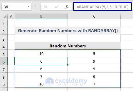
You will get an array of random numbers from numbers 5 to 10 residing in 5 rows and 2 columns with the RANDARRAY function in Excel.
Download Workbook
You can download the free practice Excel workbook from here.
<< Go Back to Random Number in Excel | Randomize in Excel | Learn Excel
Get FREE Advanced Excel Exercises with Solutions!


Hello Team,
I have posted a problem at [email protected]
Though I have solved that problem but I am not fully satisfied with my approach. I have attached my solution too in the 2nd sheet of the Test File but plz do not look at my solution in the beginning otherwise it may hinder ut independent approach to the problem.
Thanks
Uday Kumar
([email protected])
Dear UDAY KUMAR,
Good afternoon! Thank you for reaching out to us. In the following section, I’ve suggested a method for handling your issue.
First, apply this formula in cell M2.
=LAMBDA(item_name,max_issue,XLOOKUP(SEQUENCE(SUM(max_issue)),VSTACK(1,SCAN(1,max_issue,LAMBDA(a,b,a+b))),VSTACK(item_name,""),,-1))(H2:H5,I2:I5)Formula Breakdown
In this formula, item_name refers to the cell range H2:H5 of your provided worksheet, and max_issue represents the cell range I2:I5 of that worksheet.
XLOOKUP(SEQUENCE(SUM(max_issue)),VSTACK(1,SCAN(1,max_issue,LAMBDA(a,b,a+b))),VSTACK(item_name,””),,-1)) → This part of the formula will generate the Item Names according to their maximum issue number.
(H2:H5,I2:I5) → This part is required for specifying the cell ranges for item_name, and max_issue parameters of the formula.
After applying this formula, you will get an output like this in your worksheet.
Now, select these cells and copy them. Later, paste them as values in the same location.
Now, apply the following formula in adjacent cell N2 and drag the Fill Handle up to cell N32.
=RAND()After that, select the data of Column M and Column N. Then, go to the Sort & Filter option from the Home tab and choose the Custom Sort option from the drop-down.
A dialogue box named Sort will appear on your worksheet. In the Sort by field, select Column N. You can keep the other fields unchanged. Finally, click OK.
Lastly, select the entire Column N and delete it.
After following these steps, you will have a randomized list of Item Names for a month as demonstrated in the following image.
I sincerely hope that this resolves the issue that you are facing. If you need any further assistance, please let us know. Have a great day!
Regards
Zahid Hasan
ExcelDemy
Dear Uday Kumar,
We are working on your problem. We will appreciate you to post your problem in our ExcelDemy Forum.
Regards
Shamima Sultana
Project Manager | ExcelDemy